
This blog covers some of the functionality of the AlteryxPrescriptive Tool: Simulation Sampling.
I’ve been fortunate enough to work on an inventory modelling project for the last few months. This has allowed me to test the tools functionality, convince the managers of its robustness followed by using it on a day to day basis.
I will try to cover most of the tool’s functionalities down below, starting with a summary of the tool, followed by how to set it up and use it.
I’ll finish with some use case examples and provide you with a link to download the Alteryx workbook. Enjoy!
Summary
The simulation sampling tool can generate (simulate) numbers according to a set distribution, a distribution build around a data input, or sample directly from a data (one or multiple columns at the time).
The use of ‘’seeds’’ allows us the reproduce the sampled data at any time, assuming the inputs remain the same, and these seeds are appended to the data to allow for traceability.
A packaged Alteryx workflow containing all examples below can be downloaded from:
https://data.world/robbin/the-simulation-sampling-tool-in-alteryx
Let's set it up!
The tool is part of the Alteryx Predictive package. If you haven’t installed it already, go to options > Download Predictive Tools to start the installation.
Once installed, the Simulation Sampling tool can be found under the light blue Prescriptive tab. Or you can use the search bar to find it.

How can we configure it?
The tool can run either with or without inputs into the D and/or S anchors. Let’s start by running it without changing any settings or adding any inputs into the tool:
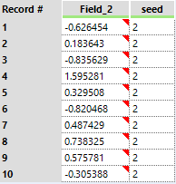
Cool! It has generated data without doing anything. This isthe general data structure of the output of this tool, it will have one ormultiple data fields and one seed field.
Let’s move on to the different settings inside the tool. The configuration pane has two tabs, the first tab allows you to select the:
- Sampling mechanism < Simple Sampling or Stratified Sampling >*
- Chunk size <the maximum data size to evaluate at one time and maximum strata size in the case of Stratified Sampling>*
- Seed <the random seed used to generate the data, allows for reproducible data>
- Number of Iterations <rows of data to generate>
- Sample Parametrically <from a distribution>
- Sample from Data <connected to the D input>
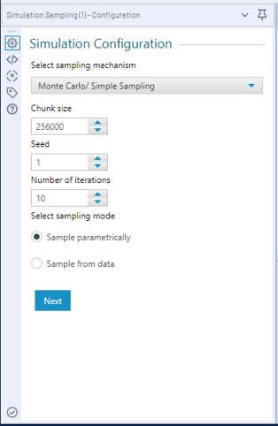
* For general use cases, Simple Sampling and default Chunk size will suffice.
In short, in simple sampling (or Monte Carlo Sampling) all data is treated as equally important, like randomly drawing a number from a bucket containing.
In stratified sampling, the data is divided into different groups (strata) and each data point can only belong to one group (stratum).
In the Simulation Sampling tool, the group size is determined by the Chunk size. Please refer to further resources such as: https://en.wikipedia.org/wiki/Latin_hypercube_sampling and feel free to reach out if you have any questions.
The second tab will change according to the selected sampletype. Let’s stick with the default settings for now and move to the second tabto check our options for the parametric sampling first.
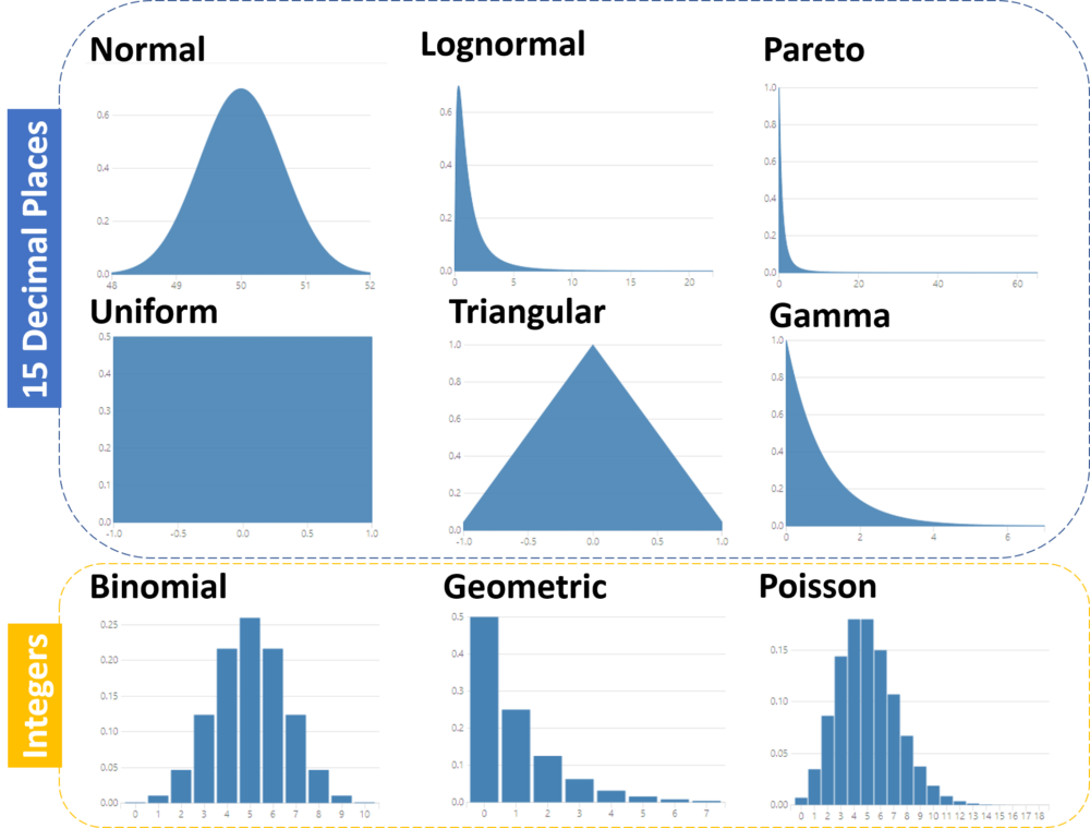
1.Parametric sampling allows us to pick a distribution, set its parameters and enter bounds (limits) for the tool to generate data from.
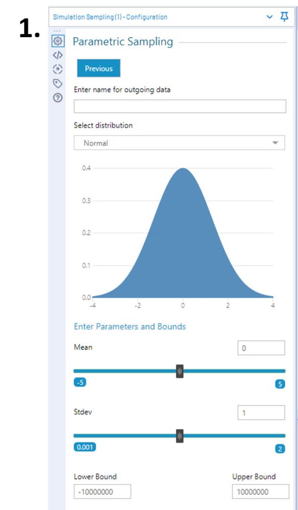
There are nine different distributions to pick from, and changing the parameters give you a visual representation of what they look like.
This means, in practice, if you set the iteration count high enough and you plot your simulated data it will be a close representation of the image.
The lower and upper bound can be set to allow for rejects of samples, i.e., using the default normal distribution as an example with a lower bound of -10000000 and upper bound of -10000000.
In the (unlikely) event that -10000001 gets sampled, it will be rejected. However, if you set it to -3 and 3, anything larger than 3 or smaller than -3 will get rejected and re-sampled. So, leave them at the default if you do not want to set limits, otherwise adjust them.
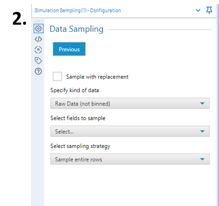
2. Sample from Data allows you to sample directly from all the data connected to the D anchor of the tool.
Ticking or unticking the sample with replacement is self-explanatory. We can compare it to drawing a random number from a bucket and we either put it back into the bucket after we noted the number (sample with replacement), or we leave it out (sample without replacement).
The ‘’Specify kind of data’’ allows you sample from the Rawdata or to add bins (IDs) manually or pre-added appended to the data. Pleasenote that if bins are selected, the simulation sampling tool will draw from thebin column rather than the data.
The ‘’Select fields to sample’’ will contain all availablenumeric fields to sample from.
The ‘’Select sampling strategy’’ allows you to ‘’sampleentire rows’’, i.e. if you have multiple fields to sample from it will draw arandom ROW number (let’s say row five) and the simulation will return row fivefor each of the selected fields. This can be useful if you always want acombination of linked numbers (such as sales and profit) to be returned.
The ‘’Sample each column independently’’ will, as the optionimplies, randomly sample from each column independently.
The last option ‘’Sample from best fitting Distribution’’allows you to set one or multiple distributions and the tool will find the bestfit to then sample from.
Turns out, to my own surprise, that there are quite a few options to tweak, which allow us to find the best possible solution for your problem.
Let’s move on to the actual interesting stuff, use cases.
Use Cases
- Dummy data generation, based on business dataand/or set limits
- Monte Carlo simulations
- Testing ‘’what if?’’ scenarios
I’m sure there are many more use cases, but these are the three I could think of and have used most frequently in the past few months.
The Alteryx workflow for all the use cases below and examples above can be downloaded from:
https://data.world/robbin/the-simulation-sampling-tool-in-alteryx
I recommend using the workflow to follow along the use cases below.
Dummy Data generation
From Business Data
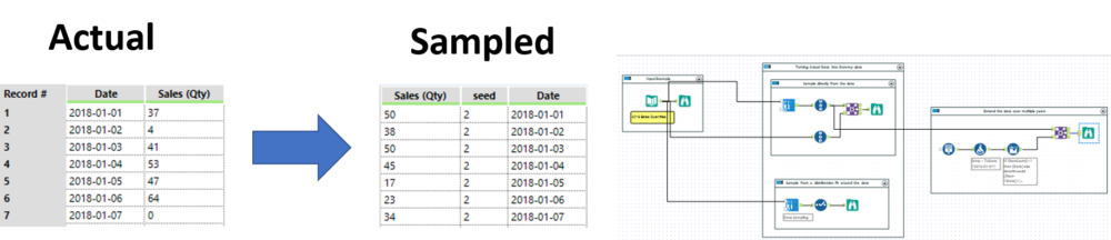
Dummy data generation made easy: connect actual numbers to the tool, sample X amount of iterations with or without replacement. This basically shuffles around the data and puts them in a random order.
If you rather not use the actual numbers, you can fit a distribution around your actual data to sample from.
Furthermore, the sample with replacement allows you to extend one year of data over a few more years if so desired.
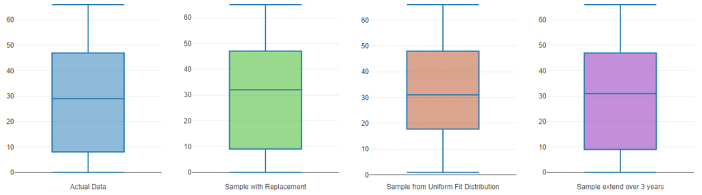
Comparing the distribution of the Actual vs. the Sampled data allows you to verify if results are as desired:
From Set Boundaries/Business Limits
Up next is an example of feeding limits or bounds to the simulation sampling tools in order to generate data.
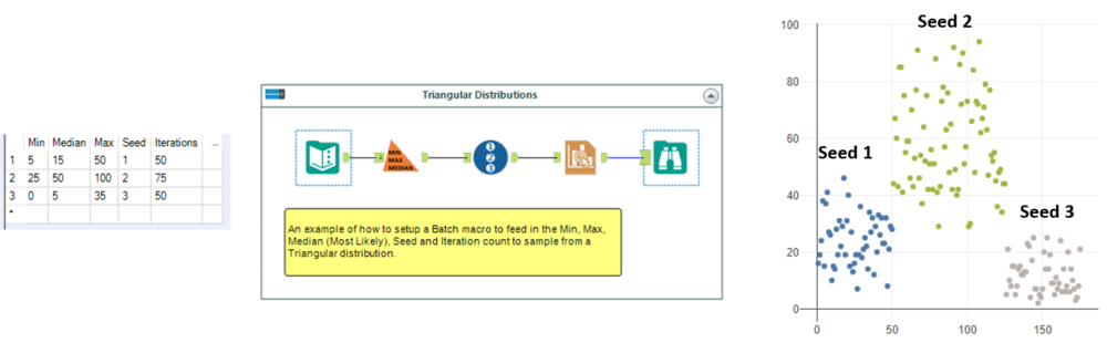
As an example, I’ve picked the Triangular Distribution and build out a simple batch macro that allows you to insert a list of numbers (Min, Median/Most Likely, Max, Iterations and Seed) to generate a set of data sampled from within those bounds.
The image below shows you the three different seeds, iterations and bounds yield in different ranges of data.
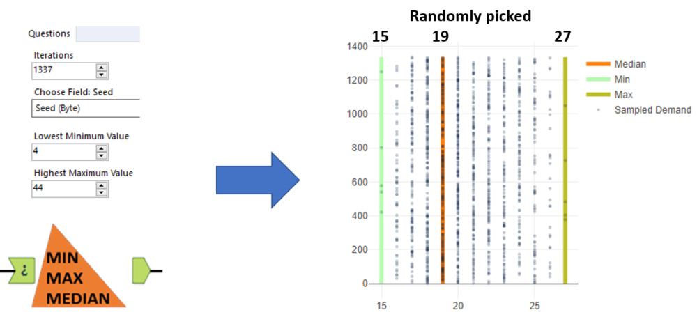
Taking it one step further, you can add more randomness to your sampled data by using distributions to generate your boundaries of your triangular distributiom.
We use a uniform distribution to generate you Min, Median and Max for the Triangular distribution.
In this example macro, we can set limits for the lowest possible value (Lowest Minimum Value) and maximum possible value that can be picked to go into the triangular distribution.
The tool will output your sampled demand appended with the pre-sampled triangular distribution bounds.
And the beauty of all the above examples are: you can reproduce the random samples if you maintain the same Seed.
In other words, if I run and save a sample of data using seed 55 and I run this again a few weeks later, with identical configuration, it will return me the same data.
Monte Carlo Simulations
In short, Monte Carlo simulations help you to visualise a whole range of possible outcomes to get a better idea of options and risk.
Now this is a very vague description so let’s see if I can put it into a verbal example.
Let’s say we have a forecast of phone sales set by management. Usually, those are at a rate or a total for the month.
Can we provision all the parts in time to make these phones? Are the chargers from the supplier going to arrive in time? How do we translate a rate or monthly total into a day to day demand?
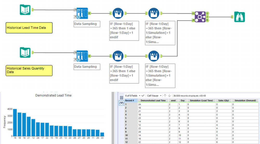
Monte Carlo Simulations allow us to provide valuableinformation to help answer these questions by using historical data.
We can use typical historical daily sales quantities, randomly sample from it and distribute them over the future days until our Monthly quota is met.
Likewise, we can use the historical delivery performance of parts from suppliers to generate a bunch of lead times of part orders and arrivals.
Each of the above sampling solutions can be run over a reasonable large amount of seeds or iterations (let’s say 100 times your sales year) and can be married up to create 100*100 = 10,000 different combinations of demand and supplier information.
Of course, more information can be added to continue to build out the relevant information required to make more informed decisions on Stock levels and order information or even feed the data into inventory modelling (which is too extensive to cover in this blog and will follow on a later date as a separate topic).
What if? Scenarios
This topic is a combination of the above two use cases, where we can use historical data and tweak things up, down, stretch, or shrink to show us what the effect would be.
This can be used to test the effect of changing certain business factors such as sales forecasts, inventory levels, profit margins, etc.
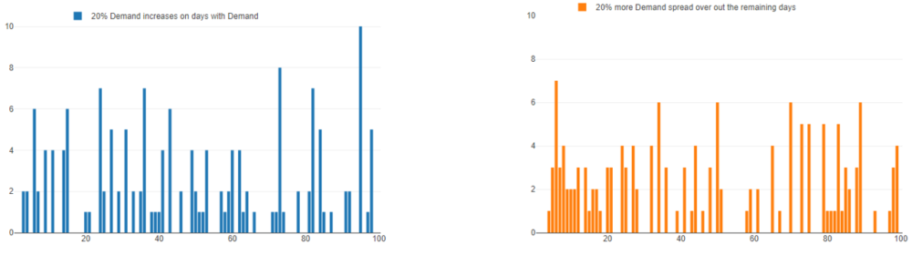
As an example, let’s use demand as our data. We have historical data and we want to visually see what possible future demand profiles would look like if:
- We increase our quantities by 20% on days that we have demand.
- We increase our quantities by 20% by spreading demand throughout the previously ‘empty’ days.
In the workflow, we use three years of historical demand. A quick inspection of the data allows us to remove 20% of the total historical records (~219) which were all 0. And for the first ‘’what if?’’ scenario we simply multiple all records by 1.2.
As you can see in the charts below, it is easy to tell the difference and if desired you can run multiple seeds to generate a range of possible outcomes for both cases.