


In this blog I will walk through how you can use Alteryx's built in Simulation Sampling tool to build a model to help optimise management of inventory (i.e. stock) levels.
The business problem
In a retail environment, good inventory management is critical for a business' success.
Levels of inventory should be managed so that shortages are minimised. Conversely, there are benefits to keeping low inventory levels - inventory is capital tied up in something which must be bought to not make a loss, it incurs storage costs, it may depreciate, etc.
So in simple terms, the risk of shortages must be balanced against the risk of keeping excess inventory to optimise the inventory levels.
Re-order point
One important aspect of inventory management this blog focusses on is the optimisation of the re-order point.
The re-order point is the level of inventory which triggers the purchase of more inventory from the supplier. So say for a clothes shop, the re-order point for a particular brand of jeans is set at a quantity of 100. Every time the number of jeans on the shelf drops below 100, the shop will order more jeans in from the warehouse.
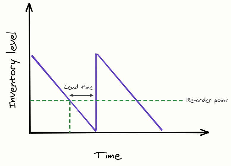
So going back to the business problem, setting a suitable re-order point is crucial to maintaining a suitable level of inventory over time. It is complicated as there is a lead time between re-ordering inventory and when it arrives to your shop. Ideally, you'd like a low re-order point - so average inventory levels are low - which also will ensure demand is filled between the day at which the re-order is made and when the re-order arrives for selling on the shelves.
However, in real life scenarios it is difficult to predict what the demand will be in this period. What if there is randomly a huge unforeseen increase in demand for a few days? What if there is nothing? How do you weigh up these risks to help decide on a suitable re-order point? Well, that is how Monte Carlo simulations can help.
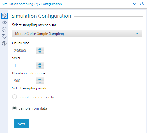
Monte Carlo Simulations to optimise re-order point
In short, in simple sampling (or Monte Carlo Sampling) all data is treated as equally important, like randomly drawing a number from a bucket.
Robbin Vernooij in his comprehensive blog on the Simulation Sampling tool here, where he covers how to configure the tool and different use cases
By using historic daily sales data for a given product, we can use the Monte Carlo method to return X rows of randomly sampled data. These rows can then be used as the sales demand forecast for the next X days.
This process can then be repeated to generate multiple demand forecast simulations. As the data is chosen randomly, different forecasts will exhibit different behaviours; how different they are depends on the distribution of the original sales data.
Each demand forecast can then be plugged into a simple model which iterates through the forecast days sequentially to calculate changes in inventory over time. Inventory decreases as it sold and increases as re-orders arrive.
Here's a step-by-step high level overview of the process
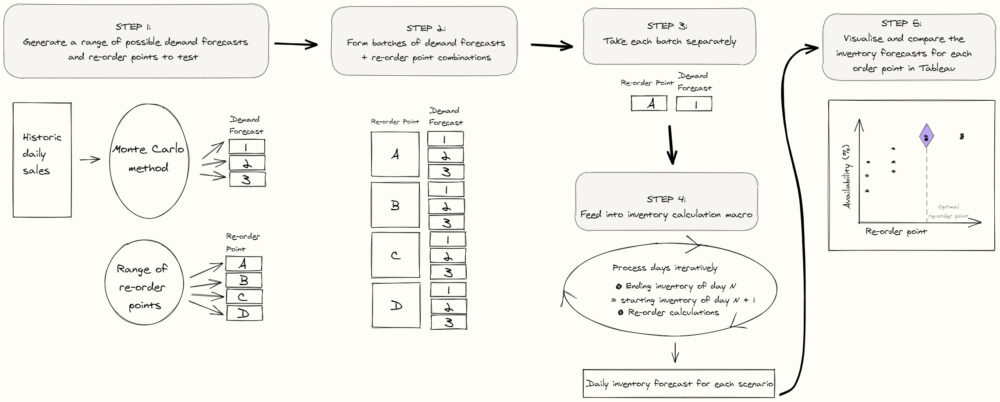
The key variables in the model include:
- Re-order point (varies from batch to batch - see diagram above)
- Re-order inventory amount (fixed value in this example)
- Starting inventory level (fixed value in this example)
- Delivery lead time (fixed value in this example)
For the iterative calculations (step 4 in diagram), each day's ending inventory by subtracting the demand forecast from the starting inventory. The ending inventory is then considered the starting inventory for the next day.
A condition is set to re-order inventory - which means in Y iterations (equal to delivery lead time) the ending inventory level will increase by a specified re-order inventory amount.
From analysing the model's outputs for all of the simulations, we can see a realistic spread of how well the inventory can be maintained in the future with the chosen re-order point. This includes under both best and worst case scenarios. This whole process can then be done with different re-order points to estimate the different risk profiles, from which we can make an informed decision on the re-order point to choose.
Putting it into to Alteryx
Now we have an idea of how it will work, it is time to put it into practice. Below is the finished process which I will walk through step by step. Jump to download link here.
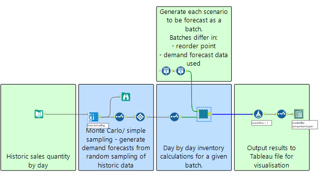
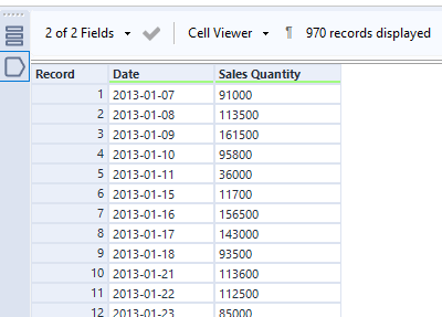
First step is to get the historic sales data grouped by day. This will be used to generate future demand scenarios.
This is then fed into a Simulation Sampling tool (found in the Prescriptive tool tab). In this example workflow, I want to do 30 simulations of 30 days for each re-order point. So naturally you might think to repeat this process 30 times for each re-order point.
However, with the Simulation Sampling tool, as well as many other tools with an R or Python backend, the act of loading up the tool each time is a major performance bottleneck. So it is more efficient to instead run the tool once, generate 900 random values and then split those into batches of 30 X 30.
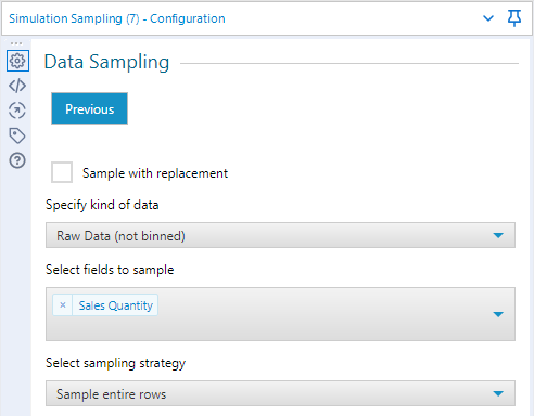
This then returns 900 random rows taken from the sales data. Via a Tile tool with Equal Records selected, the 900 rows can be separated into 30 batches.
These batches are then inputted into the batch macro, which acts as a container to run the iterative macro inventory calculations by batch as opposed to in one go.
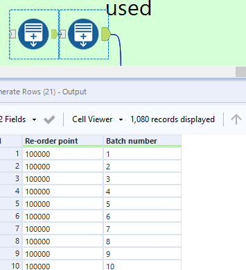
The control parameter for the batch macro helps achieve this and also updates the re-order point for each batch. The combinations of re-order point; batch number for the control parameter input are created with Generate Rows, as shown below. Effectively, each of the 30 batches are processed with each of the re-order points. In this example there are 36 re-order points so 1080 (36 *30) batch scenarios are run in total.
Within the batch macro, the control parameter updates the order point via an Action tool with each iteration.
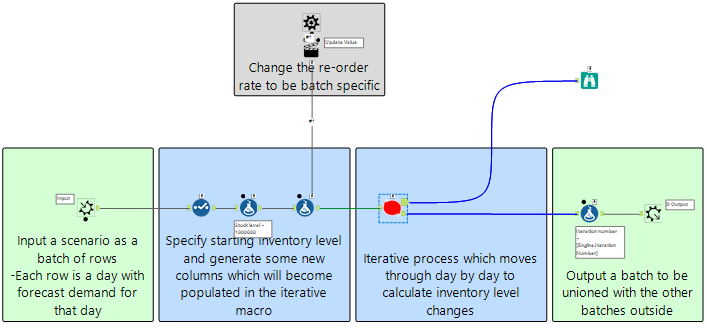
The orange macro in the image above is where the inventory changes, including re-orders, are processed day by day for a given scenario batch.
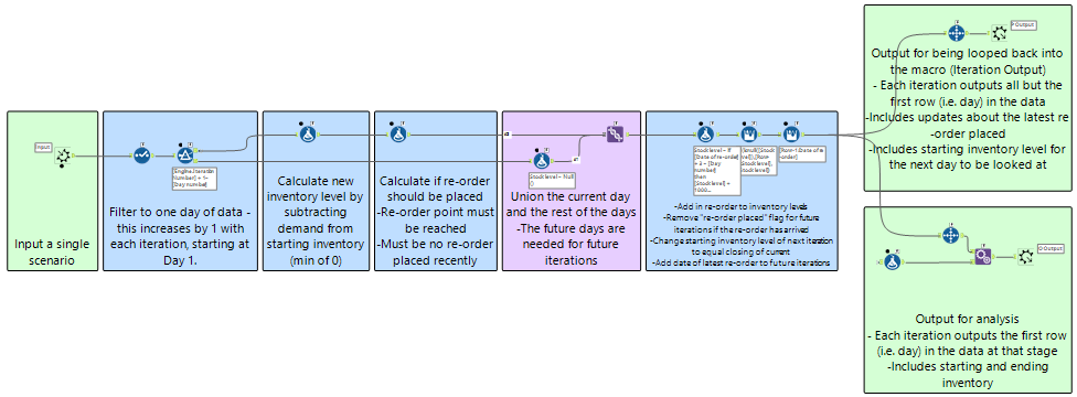
The iterative macro is fairly simple with only a few different tools used. It processes days sequentially as the starting inventory must equal the ending of the previous day (i.e. iteration).
A flag is raised if the re-order point is reached when the current inventory is calculated by subtracting forecast demand from starting inventory. If it is still above the re-order point, nothing will happen. If it is below, the flag raised and the re-order delivery date (iteration number + 3 in this example) will be passed on to future iterations via multi-row formulae.
Then, for iterations where the delivery is due, the inventory will increase by a set amount (1000000) and the re-order flag deleted. Checking the flag is needed as a pre-requisite for a re-order: for a given iteration, a re-order should only be placed if the flag is not raised - otherwise a re-order in en route.
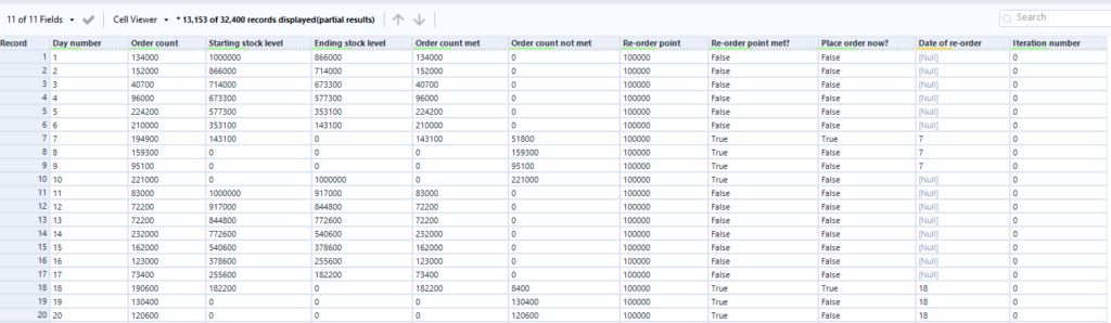
Finally, all iteration outputs for every batch are unioned and saved as a single file.
Analysis in Tableau
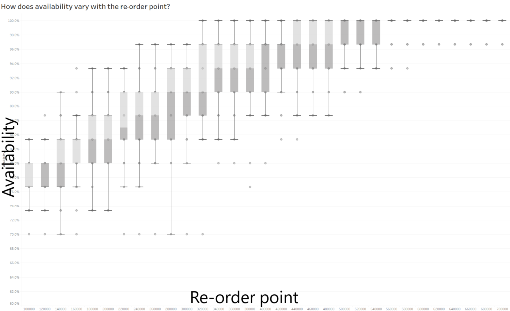
By outputting the results into Tableau, it is easy to visually compare how each inventory levels fare for each re-order point and how reliably they do so.
One method is to plot availability (% of days where all orders are filled) against re-order point. The distributions of availability for each order point are important for showing risk and the probabilistic nature of what could happen. A box plot is well suited for this as you can quickly compare best and worst case scenarios for re-order points via the whiskers and how variable scenarios are via the box widths (IQR).
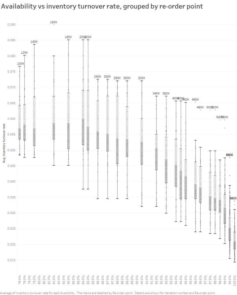
Another option would be to compare re-order points by metrics such as inventory turnover rate, which can be a useful measure of a business' efficiency in moving stock. In this example, you can see that the turnover rate is low with a very low re-order point as there are frequent shortages whereas at high re-order points it is low because there is overstocking.
A third and final chart is looking at availability against the average inventory level. This shows clearly the trade-off between inventory levels (and related costs) to being able to fill orders.
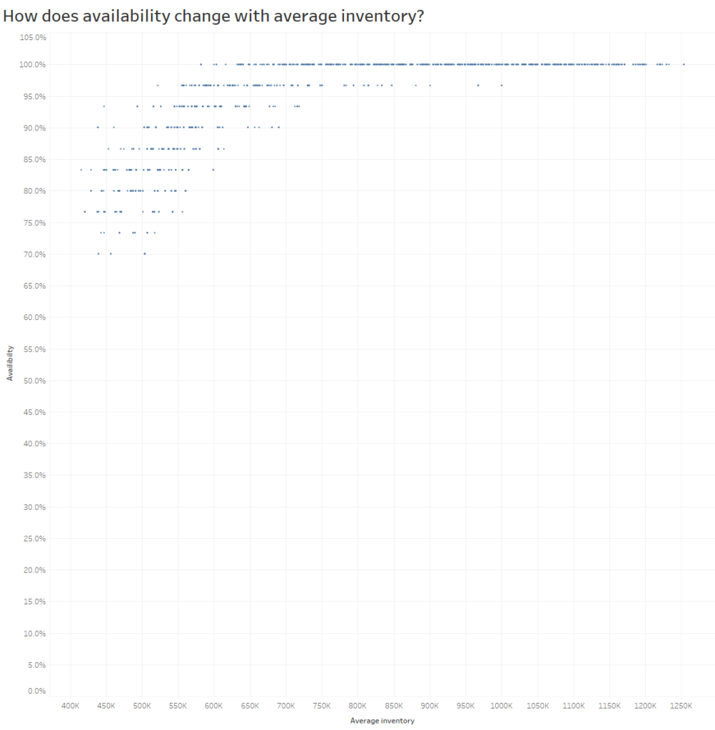
These types of charts can aide business decision makers in weighing up the costs and benefits of different re-order points.
What could be improved?
The model we have walked through makes some assumptions for the sake of simplicity. Some of these could be changed in an iteration of the model to make it more accurate:
- Lead time forecast is constant in current model
- Like with demand forecasting, using the Monte Carlo method on historic lead time data could be used to give realistic variability.
- Incorporate trend into the demand forecasting
- The model assumes that there are not any significant patterns over time - i.e. trend, seasonal, and cyclic - in the historic sales data. I filtered the example data to only the last 4 years as a crude means of reducing the effects these could have on the forecast.
- Manual inspection of the data is one way of developing bespoke rules for the model - e.g. Thursday and Friday typically have 2 X the sales of the other days so sample them separately.
- Another route could be to use conventional time series forecasting methods such as ARIMA or ETS to generate a single forecast. This could then be used to enhance the current model's demand simulations e.g. get the ratio between successive days' demand and use as a multiplicative factor for the example model's corresponding forecast demands.
- Add more parameters to the model
- Safety stock is something which could easily be added if you are interested in implementing it for your business. Is there an optimal safety stock level?
- Quantifying the cost of inventory as a function of inventory level would be worthwhile. How do all of the various inventory related costs change for 1000 units vs 10,000? It would facilitate stronger conclusions on the optimal inventory management in the future.
- Add multiple products and work out if they have different optimal re-order points
- Add more options to how customers may purchase inventory
- The model currently will not drop below 0 and excess demand will be ignored. Other options such as pre-orders could be baked in e.g. a % of customers may order while out-of-stock and pick up the next available day
That wraps up the end to this blog on inventory management with Alteryx built in tools.
Please find the materials here - an Alteryx package containing the workflow and macros as well as the downloadable Tableau workbook
I hope you enjoyed reading! Please reach out to me on Twitter if you have any questions or thoughts to share.