

26 May 2017
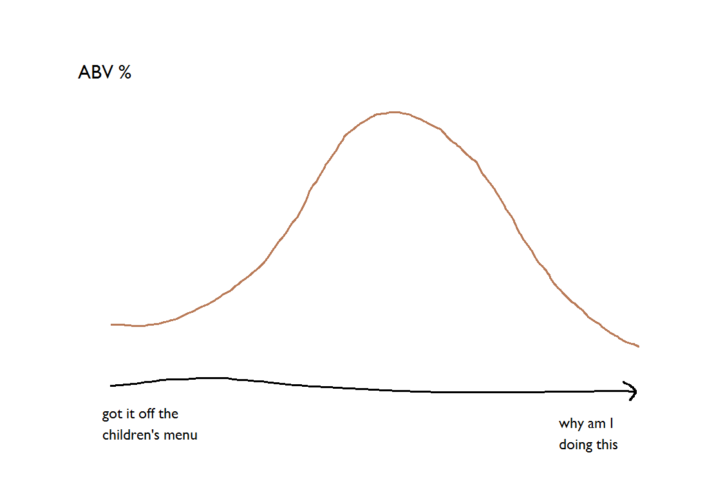
(developed and written by Gwilym and Bethany)This blog is about something you probably did right before following the link that brought you here. You’ll have looked at a variety of different factors - who posted the link? is the title interesting? does this sound relevant to your own work? does it have a nice picture? - weighed them up in your mind, and thought “okay yeah, I'll have a cheeky read of that”. Other people might have seen another factor, like the length of this blog, or the authors of this blog, and they’ll have been reminded of other blogs that they read before with similar factors which were a waste of their time. They’ll have passed over it.This kind of decision making process is something we do all the time in order to help us predict an outcome - is it worth reading this blog or not? There are loads of different predictive methods out there, but in this blog, we’ll focus on one that hasn’t had too much attention in the dataviz community: the Mahalanobis Distance calculation. And we’re going to explain this with beer.(for the conceptual explanation, keep reading! But if you just want to skip straight to the Alteryx walkthrough, click here and/or download the example workflow from The Information Lab's gallery here)Let’s say you’re a big beer fan. You’re not just your average hop head, either. You’ve devoted years of work to finding the perfect beers, tasting as many as you can. But (un)fortunately, the modern beer scene is exploding; it’s now impossible to try every single new beer out there, so you need some statistical help to make sure you spend more time drinking beers you love and less time drinking rubbish.Luckily, you’ve got a massive list of the thousands of different beers from different breweries you’ve tried, and values for all kinds of different properties. You’ve got a record of things like; how strong is it? How bitter is it? What sort of hops does it use, how many of them, and how long were they in the boil for? What kind of yeast has been used?If you know the values of these factors for a new beer that you’ve never tried before, you can compare it to your big list of beers and look for the beers that are most similar. This is the K Nearest Neighbours approach. For a given item (e.g. a new bottle of beer), you can find its three, four, ten, however many nearest neighbours based on particular characteristics. So, if the new beer is a 6% IPA from the American North West which wasn’t too bitter, its nearest neighbours will probably be 5-7% IPAs from USA which aren’t too bitter. If you tried some of the nearest neighbours before, and you liked them, then great! This new beer is probably going to be a bit like that. But if you thought some of the nearest neighbours were a bit disappointing, then this new beer probably isn’t for you. The distance between the new beer and the nearest neighbour is the Euclidian Distance.The Mahalanobis Distance is a bit different. Look at your massive list of thousands of beers again. You’ve probably got a subset of those, maybe fifty or so, that you absolutely love. They’re your benchmark beers, and ideally, every beer you ever drink will be as good as these. The Mahalanobis Distance is a measure of how far away a new beer is away from the benchmark group of great beers.To show how it works, we’ll just look at two factors for now. Let’s say your taste in beer depends on the hoppiness and the alcoholic strength of the beer. You like it quite strong and quite hoppy, but not too much; you’ve tried a few 11% West Coast IPAs that look like orange juice, and they’re not for you.Thanks to your meticulous record keeping, you know the ABV percentages and hoppiness values for the thousands of beers you’ve tried over the years. Because there’s so much data, you can see that the two factors are normally distributed: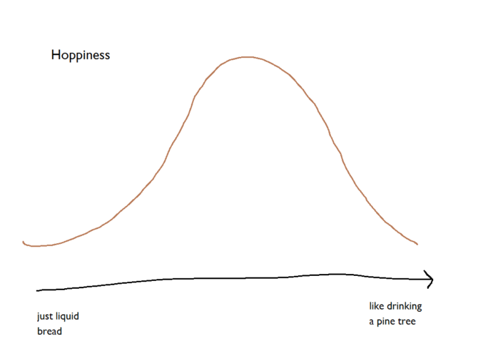
 Let’s plot these two factors as a scatterplot. Because they’re both normally distributed, it comes out as an elliptical cloud of points:
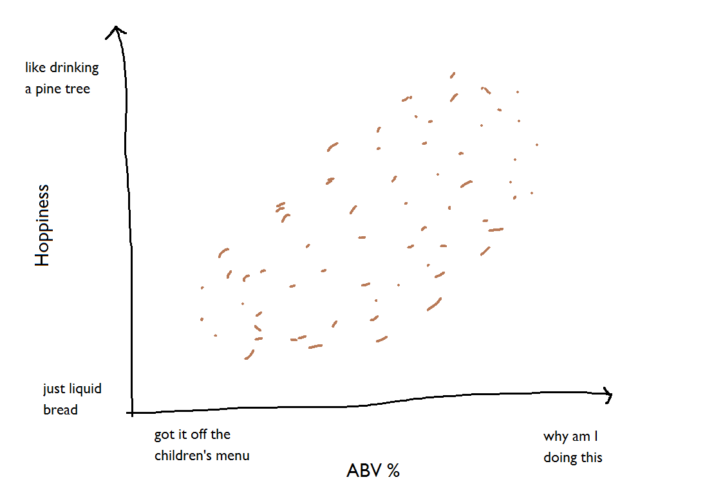 The distribution of the cloud of points means we can fit two new axes to it; one along the longest stretch of the cloud, and one perpendicular to that one, with both axes passing through the centroid (i.e. the mean ABV% and the mean hoppiness value):
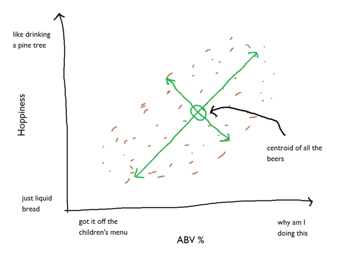 This is all well and good, but it’s for all the beers in your list. Let’s focus just on the really great beers:
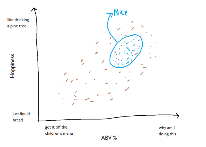 We can fit the same new axes to that cloud of points too:
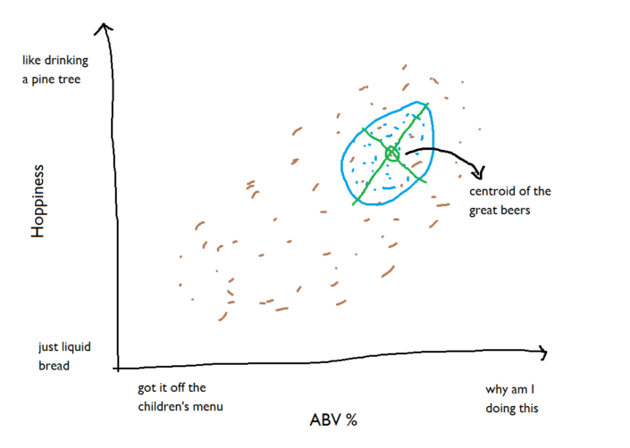 We’re going to be working with these new axes, so let’s disregard all the other beers for now:
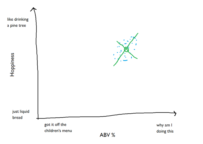 ...and zoom in on this benchmark group of beers. We can put units of standard deviation along the new axes, and because 99.7% of normally distributed factors will fall within 3 standard deviations, that should cover pretty much the whole of the elliptical cloud of benchmark beers:
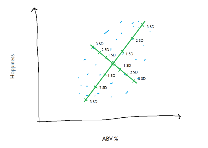 So, we’ve got the benchmark beers, we’ve found the centroid of them, and we can describe where the points sit in terms of standard deviations away from the centroid. Now, let’s bring a few new beers in. You haven’t tried these before, but you do know how hoppy and how strong they are:
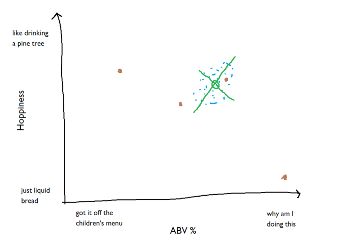 The new beer inside the cloud of benchmark beers is pretty much in the middle of the cloud; it’s only one standard deviation or so away from the centroid, so it has a low Mahalanobis Distance value:
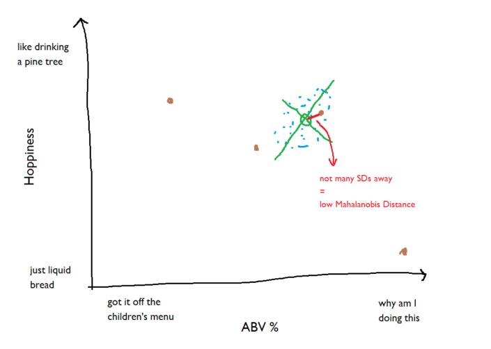 The new beer that’s really strong but not at all hoppy is a long way from the cloud of benchmark beers; it’s several standard deviations away, so it has a high Mahalanobis Distance value:
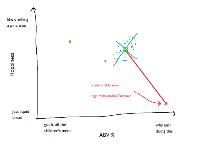 This is just using two factors, strength and hoppiness; it can also be calculated with more than two factors, but that’s a lot harder to illustrate in MS Paint.The exact calculation of the Mahalanobis Distance involves matrix calculations and is a little complex to explain (see here for more mathematical details), but the general point is this:The lower the Mahalanobis Distance, the closer a point is to the set of benchmark points.A Mahalanobis Distance of 1 or lower shows that the point is right among the benchmark points. This is going to be a good one. The higher it gets from there, the further it is from where the benchmark points are.Right. We’ve gone over what the Mahalanobis Distance is and how to interpret it; the next stage is how to calculate it in Alteryx. This will involve the R tool and matrix calculations quite a lot; have a read up on the R tool and matrix calculations if these are new to you.The overall workflow looks like this, and you can download it for yourself here (it was made with Alteryx 10.6):
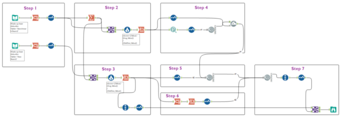 ...but that's pretty big, so let's break it down.Step 1Start with your beer dataset. Create one dataset of the benchmark beers that you know and love, with one row per beer and one column per factor (I've just generated some numbers here which will roughly - very roughly - reflect mid-strength, fairly hoppy, not-too-dark, not-insanely-bitter beers):
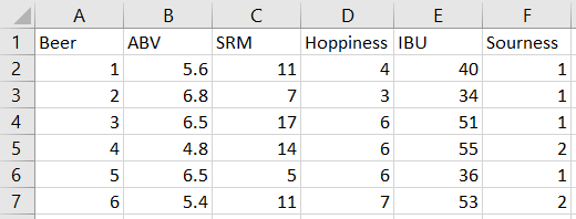 Note: you can't calculate the Mahalanobis Distance if there are more factors than records. Here, I've got 20 beers in my benchmark beer set, so I could look at up to 19 different factors together (but even then, that still won't work well). It's best to only use a lot of factors if you've got a lot of records.Another note: you can only calculate the Mahalanobis Distance with continuous variables as your factors of interest, and it's best if these factors are normally distributed. So, beer strength will work, but beer country of origin won't (even if it's a good predictor that you know you like Belgian beers).Now create an identically structured dataset of new beers that you haven't tried yet, and read both of those into Alteryx separately.Transpose the datasets so that there's one row for each beer and factor:
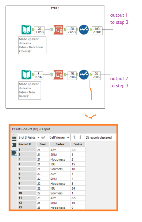 Step 2Calculate the summary statistics across the benchmark beers. Add a Summarize tool, group by Factor, calculate the mean and standard deviations of the values, and join the output together with the benchmark beer data by joining on Factor. Now calculate the z scores for each beer and factor compared to the group summary statistics, and crosstab the output so that each beer has one row and each factor has a column. You should get a table of beers and z scores per factor:
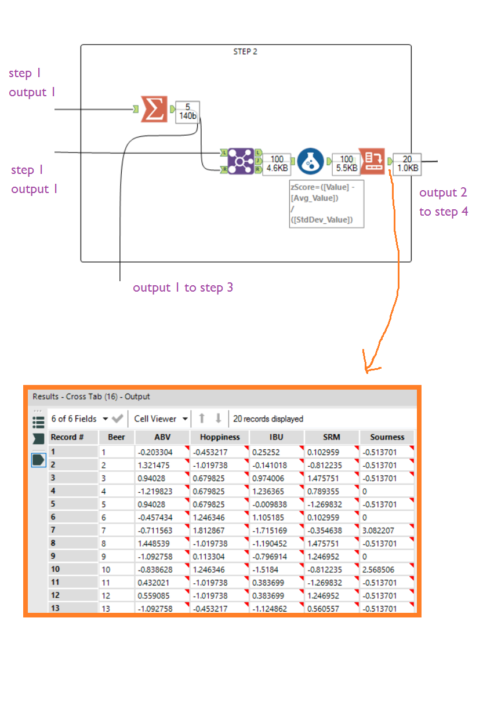 Step 3Now take your new beers, and join in the summary stats from the benchmark group. This time, we're calculating the z scores of the new beers, but in relation to the mean and standard deviation of the benchmark beer group, not the new beer group. Bring in the output of the Summarize tool in step 2, and join it in with the new beer data based on Factor. Then crosstab it as in step 2, and also add a Record ID tool so that we can join on this later.
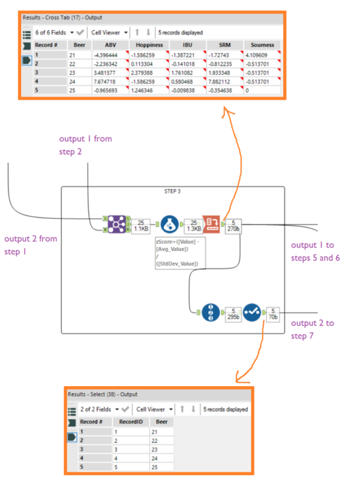 Step 4Take the table of z scores of benchmark beers, which was the main output from step 2. Add the Pearson correlation tool and find the correlations between the different factors. This will result in a table of correlations, and you need to remove Factor field so it can function as a matrix of values. Now read it into the R tool as in the code below:
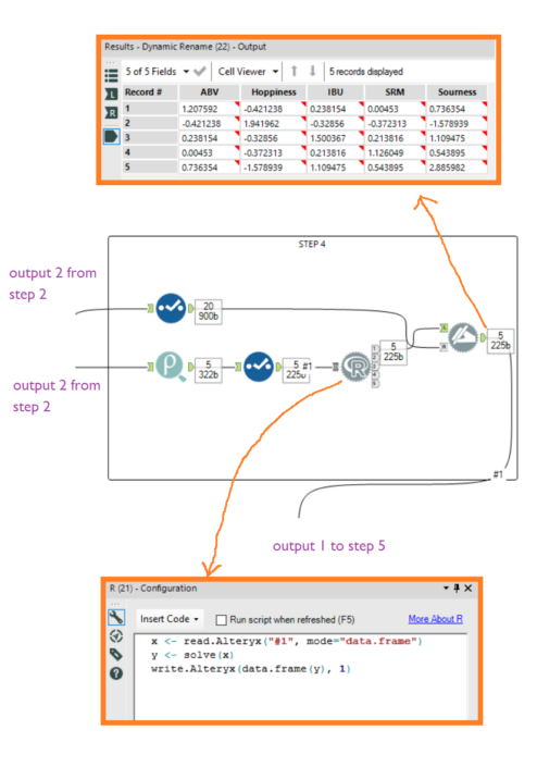 Step 5If you liked the first matrix calculation, you'll love this one. Take the correlation matrix of factors for the benchmark beers (i.e. the output of step 4) and the z scores per factor for the new beer (i.e. output 1 of step 3), and whack them into an R tool. Make sure that input #1 is the correlation matrix and input #2 is the z scores of new beers. Then add this code:
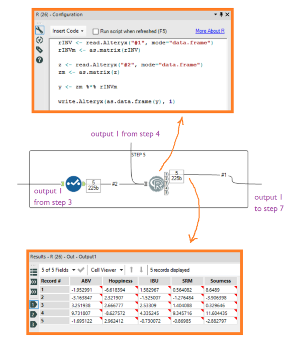 Step 6Now take the z scores for the new beers again (i.e. output 1 from step 3). We need it to be in a matrix format where each column is each new beer, and each row is the z score for each factor. First transpose it with Beer as a key field, then crosstab it with name (i.e. the names of the factors) as the grouping variable, with Beer as the new column headers and Value as the new column values. Then deselect the first column with the factor names in it:
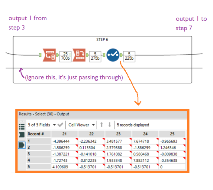 Step 7...finally! We can calculate the Mahalanobis Distance. And if you thought matrix multiplication was fun, just wait til you see matrix multiplication in a for-loop.Stick in an R tool, bring in the multiplied matrix (i.e. output 1 from step 5) as the first input, and bring in the new beer z score matrix where each column is one beer (i.e. output 1 from step 6) as the second input.Now put in this code:
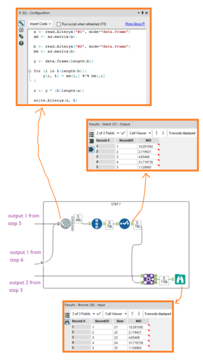 And there you have it! The Mahalanobis Distance for five new beers that you haven't tried yet, based on five factors from a set of twenty benchmark beers that you love.The lowest Mahalanobis Distance is 1.13 for beer 25. You'll probably like beer 25, although it might not quite make your all-time ideal beer list. The next lowest is 2.12 for beer 22, which is probably worth a try.The highest Mahalanobis Distance is 31.72 for beer 24. If time is an issue, or if you have better beers to try, maybe forget about this one. The Mahalanobis Distance calculation has just saved you from beer you'll probably hate....but then again, beer is beer, and predictive models aren't infallible. Even with a high Mahalanobis Distance, you might as well drink it anyway. Cheers!
 (the authors)
Let’s plot these two factors as a scatterplot. Because they’re both normally distributed, it comes out as an elliptical cloud of points:The distribution of the cloud of points means we can fit two new axes to it; one along the longest stretch of the cloud, and one perpendicular to that one, with both axes passing through the centroid (i.e. the mean ABV% and the mean hoppiness value):This is all well and good, but it’s for all the beers in your list. Let’s focus just on the really great beers:We can fit the same new axes to that cloud of points too:We’re going to be working with these new axes, so let’s disregard all the other beers for now:...and zoom in on this benchmark group of beers. We can put units of standard deviation along the new axes, and because 99.7% of normally distributed factors will fall within 3 standard deviations, that should cover pretty much the whole of the elliptical cloud of benchmark beers:So, we’ve got the benchmark beers, we’ve found the centroid of them, and we can describe where the points sit in terms of standard deviations away from the centroid. Now, let’s bring a few new beers in. You haven’t tried these before, but you do know how hoppy and how strong they are:The new beer inside the cloud of benchmark beers is pretty much in the middle of the cloud; it’s only one standard deviation or so away from the centroid, so it has a low Mahalanobis Distance value:The new beer that’s really strong but not at all hoppy is a long way from the cloud of benchmark beers; it’s several standard deviations away, so it has a high Mahalanobis Distance value:This is just using two factors, strength and hoppiness; it can also be calculated with more than two factors, but that’s a lot harder to illustrate in MS Paint.The exact calculation of the Mahalanobis Distance involves matrix calculations and is a little complex to explain (see here for more mathematical details), but the general point is this:The lower the Mahalanobis Distance, the closer a point is to the set of benchmark points.A Mahalanobis Distance of 1 or lower shows that the point is right among the benchmark points. This is going to be a good one. The higher it gets from there, the further it is from where the benchmark points are.Right. We’ve gone over what the Mahalanobis Distance is and how to interpret it; the next stage is how to calculate it in Alteryx. This will involve the R tool and matrix calculations quite a lot; have a read up on the R tool and matrix calculations if these are new to you.The overall workflow looks like this, and you can download it for yourself here (it was made with Alteryx 10.6):...but that's pretty big, so let's break it down.Step 1Start with your beer dataset. Create one dataset of the benchmark beers that you know and love, with one row per beer and one column per factor (I've just generated some numbers here which will roughly - very roughly - reflect mid-strength, fairly hoppy, not-too-dark, not-insanely-bitter beers):Note: you can't calculate the Mahalanobis Distance if there are more factors than records. Here, I've got 20 beers in my benchmark beer set, so I could look at up to 19 different factors together (but even then, that still won't work well). It's best to only use a lot of factors if you've got a lot of records.Another note: you can only calculate the Mahalanobis Distance with continuous variables as your factors of interest, and it's best if these factors are normally distributed. So, beer strength will work, but beer country of origin won't (even if it's a good predictor that you know you like Belgian beers).Now create an identically structured dataset of new beers that you haven't tried yet, and read both of those into Alteryx separately.Transpose the datasets so that there's one row for each beer and factor:Step 2Calculate the summary statistics across the benchmark beers. Add a Summarize tool, group by Factor, calculate the mean and standard deviations of the values, and join the output together with the benchmark beer data by joining on Factor. Now calculate the z scores for each beer and factor compared to the group summary statistics, and crosstab the output so that each beer has one row and each factor has a column. You should get a table of beers and z scores per factor:Step 3Now take your new beers, and join in the summary stats from the benchmark group. This time, we're calculating the z scores of the new beers, but in relation to the mean and standard deviation of the benchmark beer group, not the new beer group. Bring in the output of the Summarize tool in step 2, and join it in with the new beer data based on Factor. Then crosstab it as in step 2, and also add a Record ID tool so that we can join on this later.Step 4Take the table of z scores of benchmark beers, which was the main output from step 2. Add the Pearson correlation tool and find the correlations between the different factors. This will result in a table of correlations, and you need to remove Factor field so it can function as a matrix of values. Now read it into the R tool as in the code below:x <- read.Alteryx('#1', mode='data.frame')y <- solve(x)write.Alteryx(data.frame(y), 1)The solve function will convert the dataframe to a matrix, find the inverse of that matrix, and read results back out as a dataframe. This will remove the Factor headers, so you'll need to rename the fields by using a Dynamic Rename tool connected to the data from the earlier crosstab:Step 5If you liked the first matrix calculation, you'll love this one. Take the correlation matrix of factors for the benchmark beers (i.e. the output of step 4) and the z scores per factor for the new beer (i.e. output 1 of step 3), and whack them into an R tool. Make sure that input #1 is the correlation matrix and input #2 is the z scores of new beers. Then add this code:rINV <- read.Alteryx('#1', mode='data.frame')rINVm <- as.matrix(rINV)z <- read.Alteryx('#2', mode='data.frame')zm <- as.matrix(z)y <- zm %*% rINVmwrite.Alteryx(as.data.frame(y), 1)This will convert the two inputs to matrices and multiply them together. Because this is matrix multiplication, it has to be specified in the correct order; it's the [z scores for new beers] x [correlation matrix], not the other way around. This will return a matrix of numbers where each row is a new beer and each column is a factor:Step 6Now take the z scores for the new beers again (i.e. output 1 from step 3). We need it to be in a matrix format where each column is each new beer, and each row is the z score for each factor. First transpose it with Beer as a key field, then crosstab it with name (i.e. the names of the factors) as the grouping variable, with Beer as the new column headers and Value as the new column values. Then deselect the first column with the factor names in it:Step 7...finally! We can calculate the Mahalanobis Distance. And if you thought matrix multiplication was fun, just wait til you see matrix multiplication in a for-loop.Stick in an R tool, bring in the multiplied matrix (i.e. output 1 from step 5) as the first input, and bring in the new beer z score matrix where each column is one beer (i.e. output 1 from step 6) as the second input.Now put in this code:a <- read.Alteryx('#1', mode='data.frame')am <- as.matrix(a)b <- read.Alteryx('#2', mode='data.frame')bm <- as.matrix(b)y <- data.frame(length(b))for (i in 1:length(b)){y[i, 1] = am[i,] %*% bm[,i]}z <- y / length(a)write.Alteryx(z, 1)Each row in the first input (i.e. 'a' in this code) is for the new beer, and each column in the second input (i.e. 'b' in this code') is for the new beer. What we need to do is to take the Nth row of the first input and multiply it by the corresponding Nth column of the second input. This means multiplying particular vectors of the matrix together, as specified in the for-loop. This will create a number for each beer (stored in 'y'). Then we need to divide this figure by the number of factors we're investigating. We could simply specify five here, but to make it more dynamic, you can use length(), which returns the number of columns in the first input.This returns a simple dataframe where the column is the Mahalanobis Distance and each row is the new beer. But because we've lost the beer names, we need to join those back in from earlier. Remember how output 2 of step 3 has a Record ID tool? Well, put another Record ID tool on this simple Mahalanobis Distance dataframe, and join the two together based on Record ID. Alteryx will have ordered the new beers in the same way each time, so the positions will match across dataframes.And there you have it! The Mahalanobis Distance for five new beers that you haven't tried yet, based on five factors from a set of twenty benchmark beers that you love.The lowest Mahalanobis Distance is 1.13 for beer 25. You'll probably like beer 25, although it might not quite make your all-time ideal beer list. The next lowest is 2.12 for beer 22, which is probably worth a try.The highest Mahalanobis Distance is 31.72 for beer 24. If time is an issue, or if you have better beers to try, maybe forget about this one. The Mahalanobis Distance calculation has just saved you from beer you'll probably hate....but then again, beer is beer, and predictive models aren't infallible. Even with a high Mahalanobis Distance, you might as well drink it anyway. Cheers!(the authors)