

26 May 2017
Many of you in the world of data will have heard of matrix calculations. Matrices are the big rectangles full of numbers that often crop up in statistical analysis techniques, and doing calculations with them doesn’t work quite the same as with normal numbers. In this blog, I’m going to explain the basics behind matrix calculations without going in to too much detail (and for those of you out there who want to understand the specifics behind what I’m about to go through, I’ll include links to websites which can offer more detailed explanations).Let’s start off with a story.Imagine you work at a bar, and you need to report back to your boss the individual amounts spent on beer orders and G&T orders. You thought you’d kept on top of it all night, until you find two receipts; they have the quantity of drinks ordered, their totals, but not the break down cost:Receipt 1: 1 beer + 1 G&T = £9Receipt 2: 3 beers + 2 G&T = £22You can’t remember the costs of each drink, so you need to try and figure it out. I’m going to transport you back to GCSE maths now and talk about simultaneous equations - let’s call the beers ‘x’ and the G&Ts ‘y’. So, our problem boils down to the following set of equations: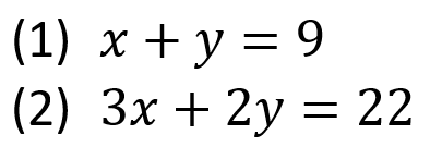 We can view this set of equations in a matrix form:
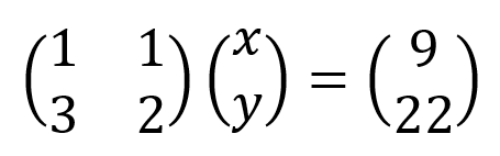 (I’ll explain how this works in a second…)I know you must be thinking right now - why would I want to do that? It looked perfectly fine as it was before! And I’d agree. This is a system of 2 equations with 2 unknown variables (x and y), so it’s pretty simple... but what happens when you’ve screwed up the whole bar tab and you have to figure out the individual cost of every single drink sold that night? Or, in maths terms, what happens when you have n equations with n unknown variables? This is where it’s nice to wrap all your equations up in a nice little matrix package. I’m not going to go in to details on how to solve this particular problem with matrices as that can get into some pretty complicated stuff pretty quickly, but this is one way matrices can be really useful!So, how does that weird bracket-y thing relate to those equations? How do I get it back to the equations I preferred before? You use matrix multiplication!
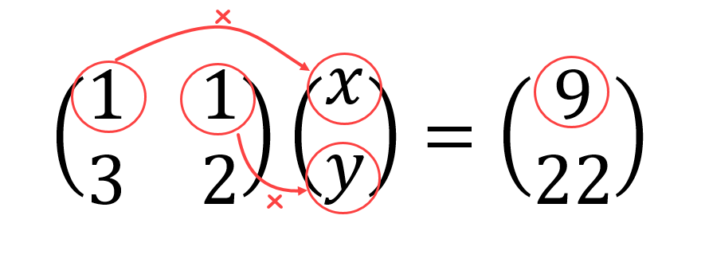 So we have:
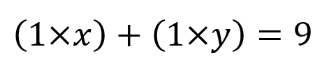 Then you do the same with the bottom row:
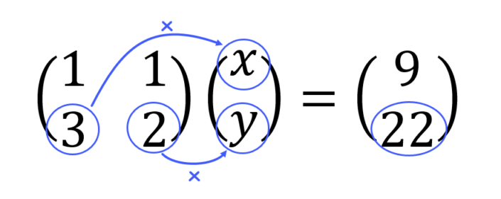 Which gives:
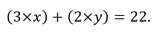 So all in all we have:
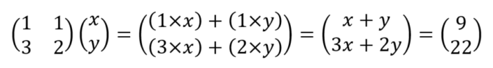 And that’s it! You just keep going until all rows in the first matrix have been multiplied by all corresponding columns in the second matrix. If we were multiplying two matrices together of dimension, say two 2×2 matrices (matrices with 2 rows and 2 columns, read “2 by 2”), you would simply repeat the same method for the second column of the second matrix. Check out this video on how this works. If you’re using R, and have a matrix A and a matrix B to multiply together, the command is ‘A%*%B’.I’m going to introduce you to a friend of mine called Rose Columns, and she’ll help you remember which way round to multiply the elements – just go along the rows of the first matrix, and down the columns of the second matrix. Nobody would ever be called Columns Rose (that’s just weird), so just remember her name and you’ll get it right every time.This a good time to point out that the order of the matrices matters when you’re multiplying – matrix multiplication is not commutative. In other words, if you have a matrix called A, and a matrix called B, then A∙B≠B∙A (the ‘dot’ here means multiplication). Additionally, you can’t multiply any old matrix by any other old matrix, their dimensions must be compatible. In our bar tab example, we’re multiplying a 2×2 matrix by a 2×1 matrix. One trick to quickly see if the order of the multiplication works is to check if the middle two numbers are the same; if they are the same, the dimension of your new matrix will be the two outer numbers together:
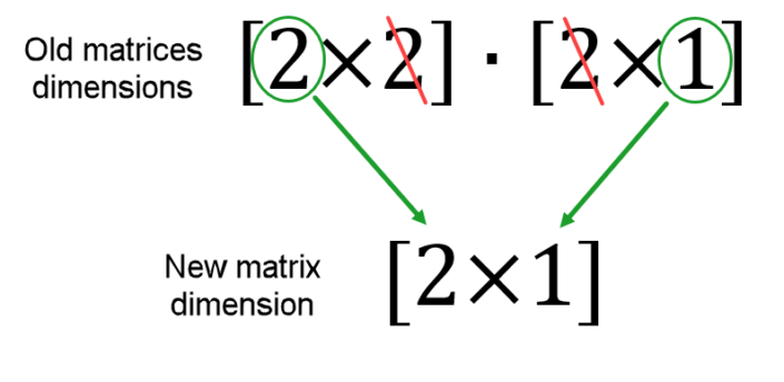 If the two middle numbers don’t match, you can’t multiply the two matrices together.
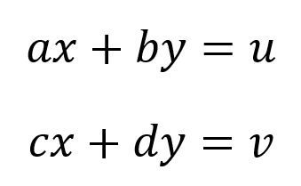 Where x and y are the unknown variables, and a, b, c, d, u, and v are known constants. This can be written in the matrix form:
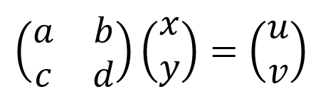 The solution to this system of equations is:
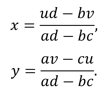 If you don’t understand how I came to this solution, check out this link. Notice that the denominator (the part on the bottom of each fraction), is the same in the solution for both x and y. This value (ad-bc) is called the determinant; if it is non-zero, then there exists a unique solution to the equations. The determinant basically determines whether it is possible to find a solution or not, hence the name. To find it in a 2×2 square matrix is really easy. Simply take the left diagonal values multiplied together and subtract the right diagonal values from it.
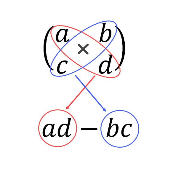 To find the determinant of bigger square matrices is a little trickier, I won’t go in to details here as this blog is just to cover the basics, but if you want to find out more I’d recommend checking out this website. We’ll need the determinant to find out the inverse of a matrix. If you want to find the determinant of a matrix, A, in R, use the command ‘det(A)’.
 . Unfortunately you can’t just do one over every element in the matrix to get the inverse, it takes a little more work than that. It’s simple enough in a 2×2 matrix, so I’ll demonstrate it with that.We have a matrix
 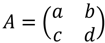 , and we want to find . First, let’s do a little shuffling of the elements inside the matrix:
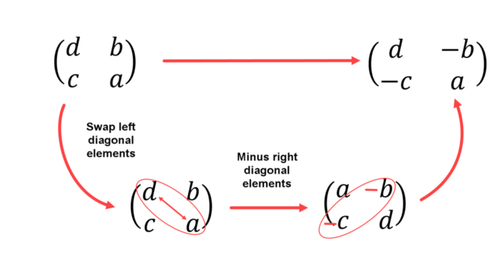 Now all we need to do is divide the shuffled matrix by the determinant:
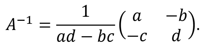 For bigger matrices it gets much trickier to do by hand, and takes A LOT of time for anything bigger than a 3×3 matrix, here is a bit of info on it. Luckily enough, there are plenty of online matrix inverse calculators for us to use, or if you’re using R, the command is simply ‘solve(A)’.Okay, now we’ve been over matrix multiplication, inversion, and finding the determinant, I’ll finish off by going over a few other basic operations involving matrices to cover a few more bases.
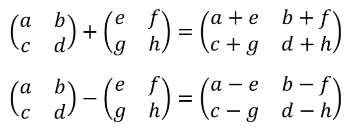
 .
. Hopefully this has addressed all your matrix needs!
(I’ll explain how this works in a second…)I know you must be thinking right now - why would I want to do that? It looked perfectly fine as it was before! And I’d agree. This is a system of 2 equations with 2 unknown variables (x and y), so it’s pretty simple... but what happens when you’ve screwed up the whole bar tab and you have to figure out the individual cost of every single drink sold that night? Or, in maths terms, what happens when you have n equations with n unknown variables? This is where it’s nice to wrap all your equations up in a nice little matrix package. I’m not going to go in to details on how to solve this particular problem with matrices as that can get into some pretty complicated stuff pretty quickly, but this is one way matrices can be really useful!So, how does that weird bracket-y thing relate to those equations? How do I get it back to the equations I preferred before? You use matrix multiplication!Matrix multiplication
This isn’t anywhere near as complicated as it sounds, all you do is multiply the rows by the columns, and add up the elements. For example, to get equation (1) you multiply the elements in the top row of the first matrix by the elements of the column matrix next to it, and add it up:So we have:Which gives:And that’s it! You just keep going until all rows in the first matrix have been multiplied by all corresponding columns in the second matrix. If we were multiplying two matrices together of dimension, say two 2×2 matrices (matrices with 2 rows and 2 columns, read “2 by 2”), you would simply repeat the same method for the second column of the second matrix. Check out this video on how this works. If you’re using R, and have a matrix A and a matrix B to multiply together, the command is ‘A%*%B’.I’m going to introduce you to a friend of mine called Rose Columns, and she’ll help you remember which way round to multiply the elements – just go along the rows of the first matrix, and down the columns of the second matrix. Nobody would ever be called Columns Rose (that’s just weird), so just remember her name and you’ll get it right every time.This a good time to point out that the order of the matrices matters when you’re multiplying – matrix multiplication is not commutative. In other words, if you have a matrix called A, and a matrix called B, then A∙B≠B∙A (the ‘dot’ here means multiplication). Additionally, you can’t multiply any old matrix by any other old matrix, their dimensions must be compatible. In our bar tab example, we’re multiplying a 2×2 matrix by a 2×1 matrix. One trick to quickly see if the order of the multiplication works is to check if the middle two numbers are the same; if they are the same, the dimension of your new matrix will be the two outer numbers together:If the two middle numbers don’t match, you can’t multiply the two matrices together.The determinant
Let’s generalise this example and use some arbitrary values. Say we now have the following simultaneous equations:Where x and y are the unknown variables, and a, b, c, d, u, and v are known constants. This can be written in the matrix form:The solution to this system of equations is:If you don’t understand how I came to this solution, check out this link. Notice that the denominator (the part on the bottom of each fraction), is the same in the solution for both x and y. This value (ad-bc) is called the determinant; if it is non-zero, then there exists a unique solution to the equations. The determinant basically determines whether it is possible to find a solution or not, hence the name. To find it in a 2×2 square matrix is really easy. Simply take the left diagonal values multiplied together and subtract the right diagonal values from it.To find the determinant of bigger square matrices is a little trickier, I won’t go in to details here as this blog is just to cover the basics, but if you want to find out more I’d recommend checking out this website. We’ll need the determinant to find out the inverse of a matrix. If you want to find the determinant of a matrix, A, in R, use the command ‘det(A)’.Inverse of a matrix
An inverse of a matrix is basically 1 over that matrix. Say we have a matrix called A, then the inverse of A is 1⁄A, it is also denoted byNow all we need to do is divide the shuffled matrix by the determinant:For bigger matrices it gets much trickier to do by hand, and takes A LOT of time for anything bigger than a 3×3 matrix, here is a bit of info on it. Luckily enough, there are plenty of online matrix inverse calculators for us to use, or if you’re using R, the command is simply ‘solve(A)’.Okay, now we’ve been over matrix multiplication, inversion, and finding the determinant, I’ll finish off by going over a few other basic operations involving matrices to cover a few more bases.Matrix Addition and Subtraction
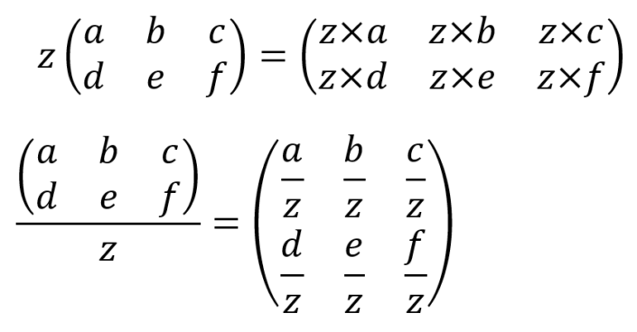
This is only possible with matrices that are of the same dimensions, and it’s as simple as you’d hope for. Simply add, or subtract, the elements which are in the same position in each matrix.Matrix multiplication/division by a scalar
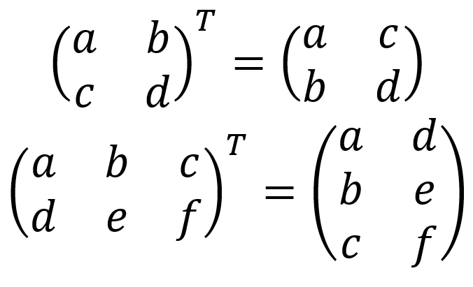
We’ve already done division by a scalar when finding the inverse of a 2×2 matrix, we divided by the determinant (multiplied it by one over the determinant). So this is also as easy as you’d hope for!Transpose of a matrix
This is something we haven’t covered at all so far in this blog, but it is always handy to know, especially since it’s so easy! All you have to do, is turn all the columns in to rows, and all the rows in to columns. N.B. If the matrix you’re doing this to is not a square matrix (i.e. the same number of rows as columns), then the dimensions of your matrix will be flipped. The transpose of a matrix A is denoted byHopefully this has addressed all your matrix needs!