


When comparing different values over time, it is sometimes good to see how the two metrics differ from each other and to highlight the change. One way of doing this is to shade the area between the two lines which helps to highlight the difference.
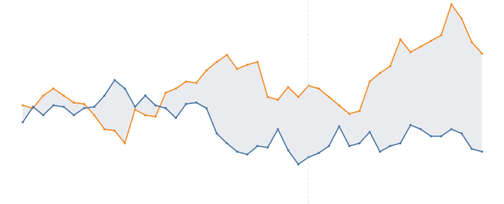
In Tableau there is no native way of doing this so we need to get a bit creative in order to achieve the desired effect. There are a couple of options, we could just have a single block colour to highlight the difference as shown in here:
How to achieve this technique is covered in the great blog post from Tim Manning which can be found here.
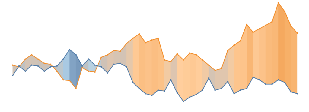
However, if we wanted to take this a step further and have the shading change depending on the size of change, we need to think about this in a slightly different way. In this blog, I will use polygons to create bars within the shaded region to show the difference between our two metrics at the same point:
The Technique
For this example, I'm going to use football data that takes a look at the change in Expected Goals for Sheffield United since they were promoted to the Premier League (Data is from FBRef.com). Don't worry too much about understand the data, I've used it as it shows the switch over so we have some different colours. Using the data from Tim's Block Shade example would work here too.
The data is structured in the following way, and I have highlighted the main fields that we are going to be using:
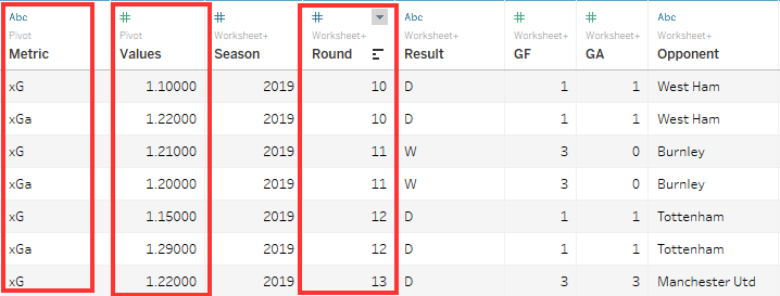
The Metric & Values field are what we are going to be comparing (the two different lines). Then the Round field will be our X axis (the overtime element).
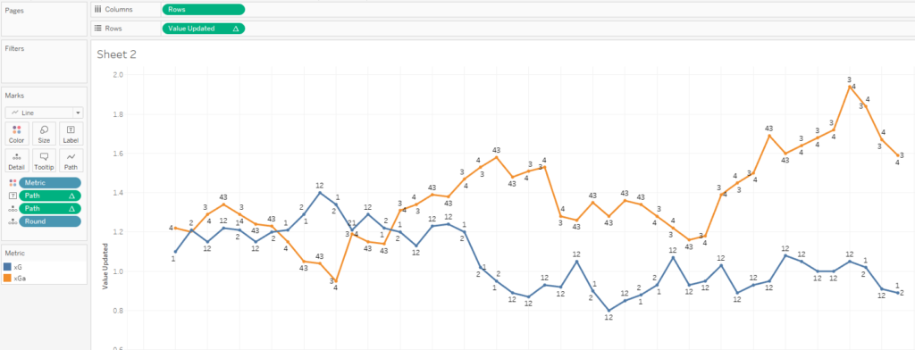
1. Create Line Chart
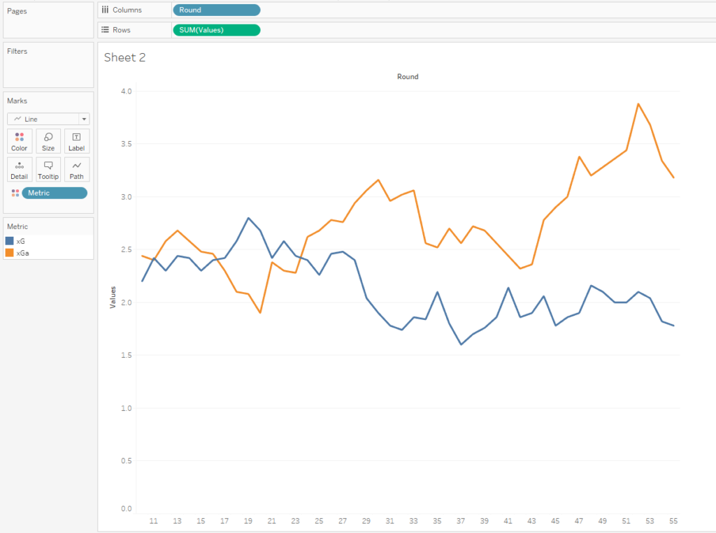
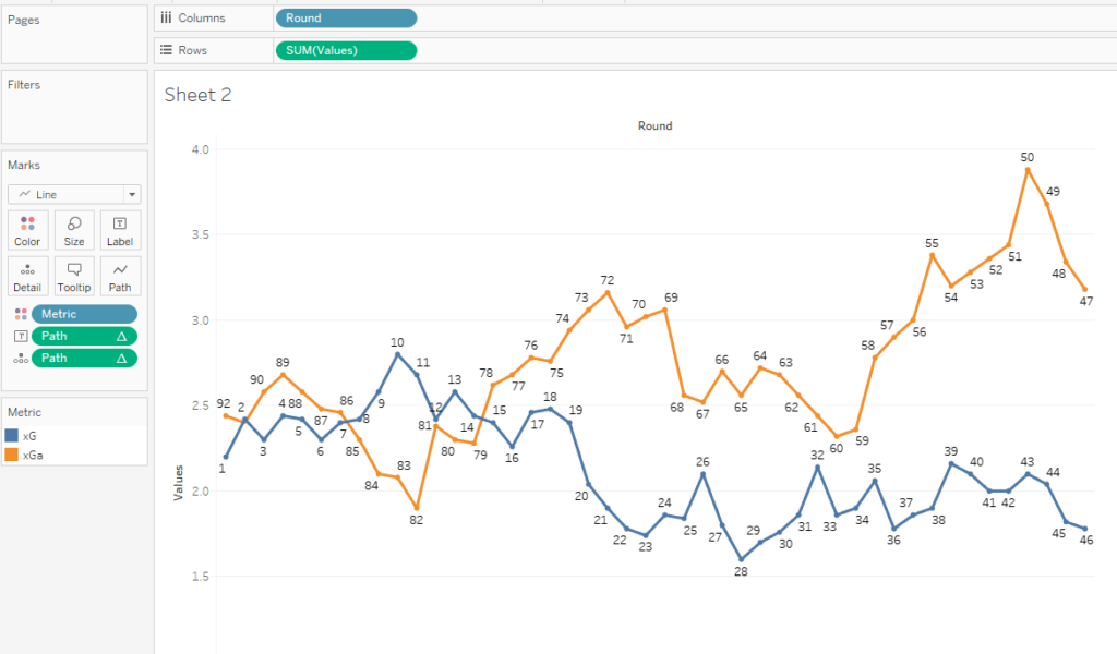
The first step is to create a basic line chart showing both of the metrics over time which should look like this:
2. Densify Data
In order to create the different coloured bars between the metrics we are going to create separate polygons. For this to be possible we need to have four different points, one for each corner of our shape. To achieve this we first need to densify our data so that we have the actual value, and the next value on the same row. For example, round 1 and round 2 on a single row.
Note, if you just want a single shade colour between the lines then this densification step isn't necessary.
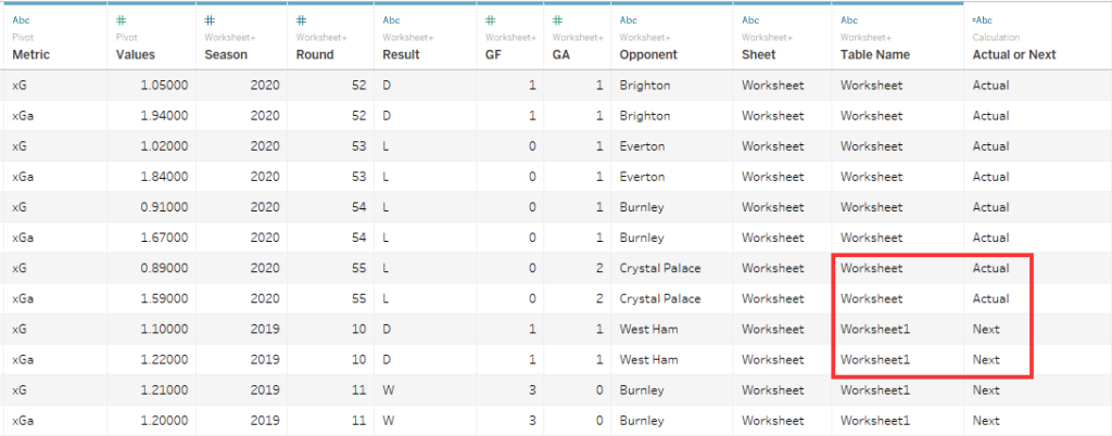
Therefore, we want to union our data source on to itself so that it is duplicated and the Table Name field is created.
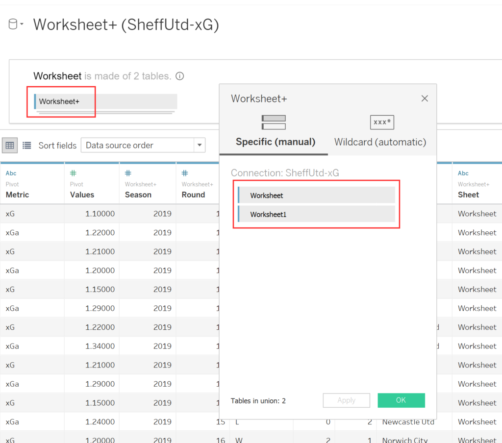
We can then update the Table Name so that it is Actual or Next using this calculation:
Actual or Next
IF [Table Name] = 'Worksheet 1' THEN 'Next'ELSE 'Actual'ENDWe now have two duplicated rows split by Actual or Next:
3. Table Calculations
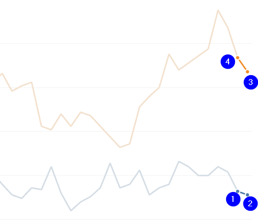
The next step is to create the different points for our polygon. We want to have a different number for each of the different corners as shown by the corresponding numbers below:
We will use different table calculations to create each of the different numbers. We will need the following calculations:
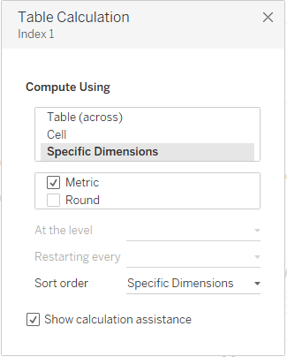
Index 1
Index()
This is used to give each of our different metrics a different number, as shown here:
I have updated the table calculation settings so that it computes on the Metric field:
Index 2
Index()
This is giving us a continuous count for each of the metrics that looks like this:
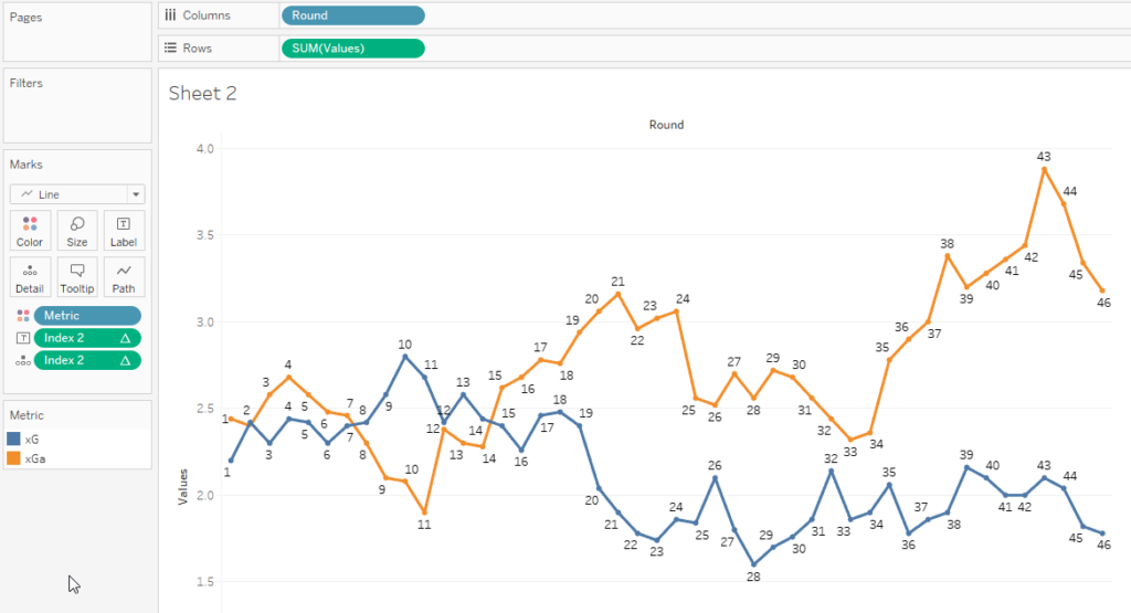
There are now changes to the table calculation setup so it is computing across the table.
Last
Last() + 1
Next we want the continuous count to be reversed so we use the last() function. Last starts on 0, therefore we need to add 1 to get the following result:
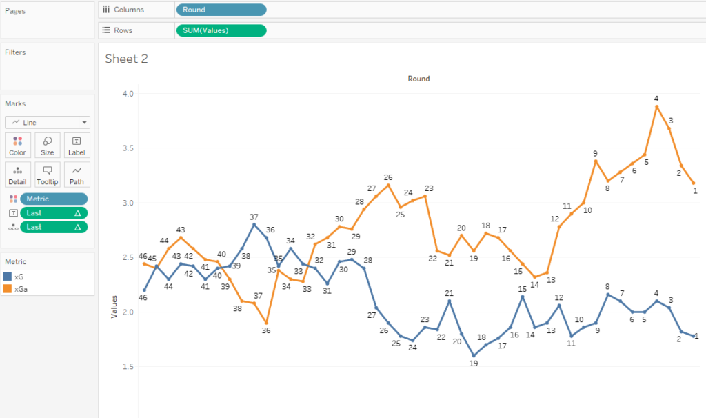
Again, no changes to the table calculation so it should be computing across the table.
Size
Size()
The final table calculation we need is to return the overall highest value. Therefore, we use the size calculation to return the values here:
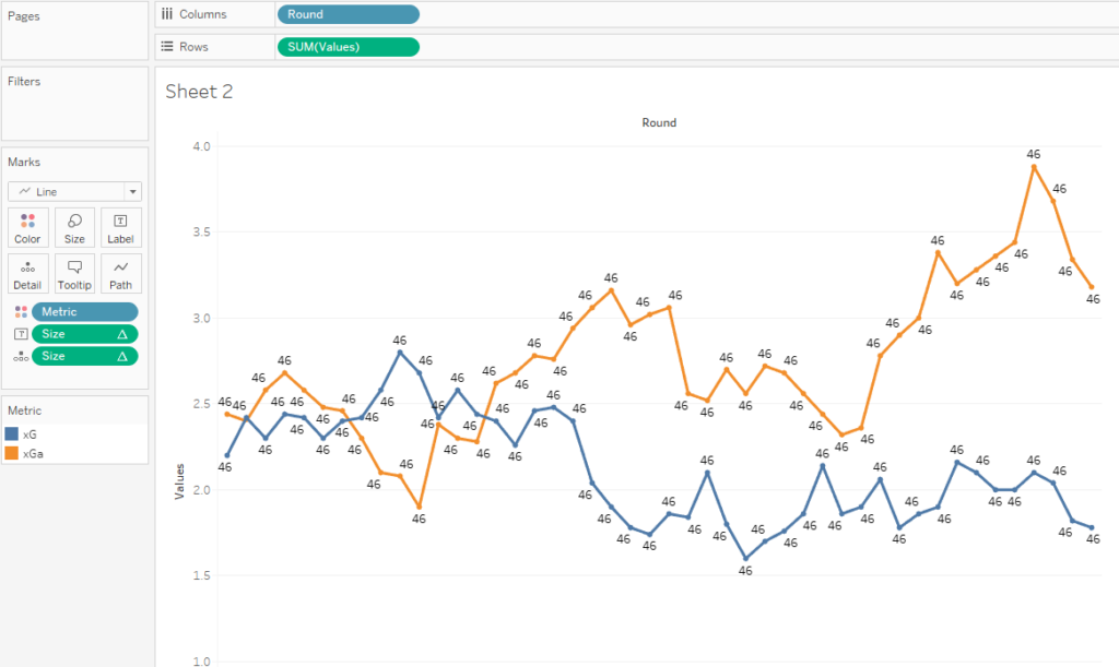
No change to the table calc again, so computing across the table works fine.
Path
IF [Index 1] = 1 THEN [Index 2]
ELSE [Last] + [Size]
END
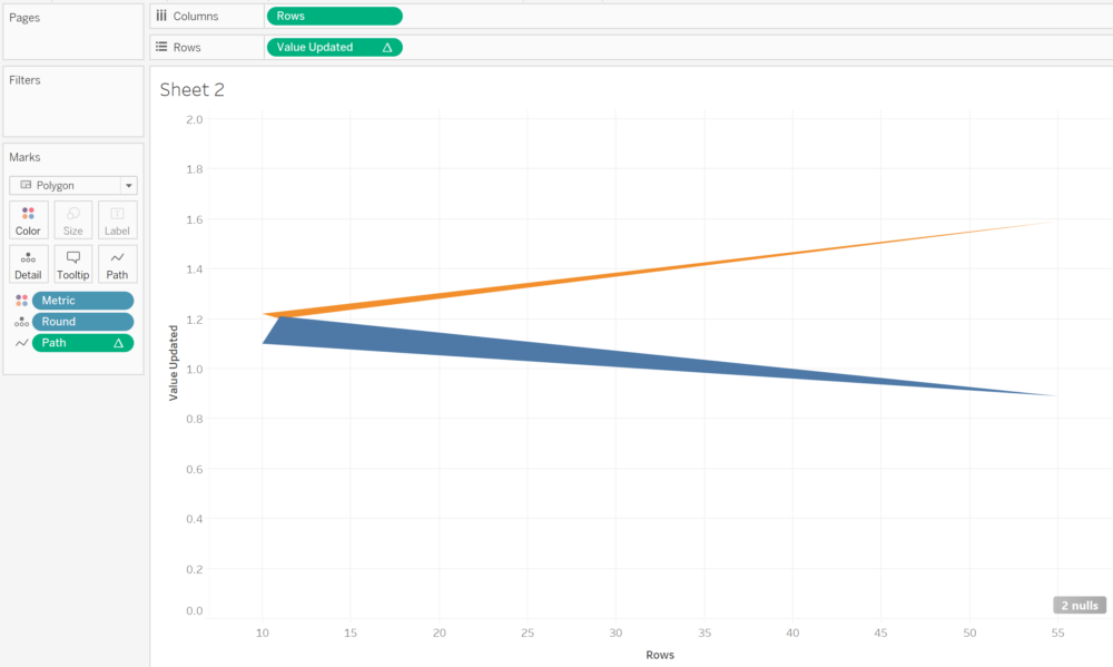
We can now bring all of these together to give us the different numbers for each point which we need to make the polygons. Notice how we have a continuous number sequence for both lines which restarts are the end of the blue line then continues onto the orange:
This is how we are going to create the shaded area polygon, as Tableau now has the route back to the start. If you put the Path field onto Path you will see the line connecting point 46 & 47 and where Tableau will draw the polygon.
Make sure you have updated the table calculation for Index 1 only just like we did previously:
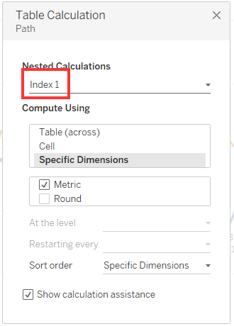
Note, you may want to change all of the other table calculations to computing using 'X'. This will stop the calculation from giving unexpected results if you were to change something in the view.
4. Update Rows & Columns
Now we have all of the Table Calculations setup, we need to make some changes to what is in our Rows & Columns shelf. This will only work if we have a Measure in both of these, therefore we need to update the Round field on Columns to get this working. We also need to adjust this because of the duplication of data earlier, so I have created a new Rows field.
Rows
IF [Actual or Next] = 'Actual' THEN [Round]
ELSE [Round]+1
END
This helps to readjust the Actual and Next values to give us the width in the Polygon. For example, if the Actual value = 1 then the next value will be 2 and so on.
For the measure on the columns shelf, we need to readjust this as the next is being skewed due to the Actual and Next values being on the same row. Therefore, we use the following calculation to make sure we are looking at the correct values:
Value Updated
IF ATTR([Actual or Next]) = 'Actual' THEN SUM([Values])
ELSE LOOKUP(SUM([Values]),1)
END
The Lookup function here allows us to look at the next value or the right side of our polygon.
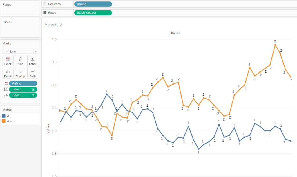
We can then replace these values on the Rows & Columns shelf so that our line chart looks like this: (Rows on rows, Value Updated on columns, and Round on detail)
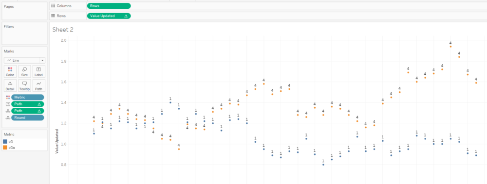
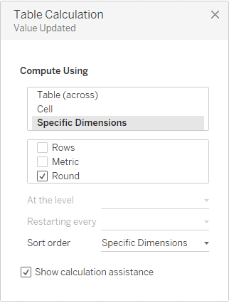
Notice how this has split our view into single dots, therefore we need to updated the Table Calculation on the Value Updated field so that it is computing on Round.
Then our line chart will look like this:
5. Create Polygons
We are now ready to create the polygons between the two different lines. First, we need to change the mark type from a Line to a Polygon, then move the Path field onto Path.
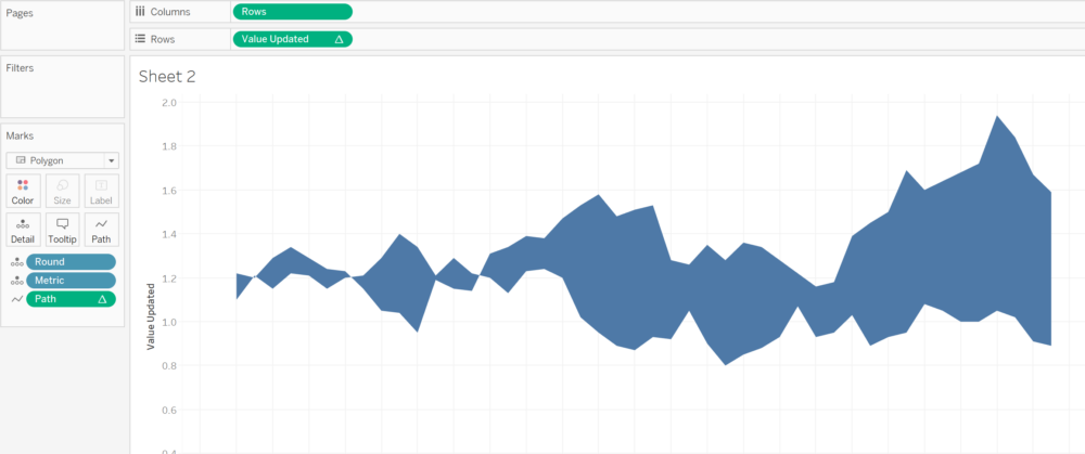
This creates two triangles which doesn't look like what we are trying to create but if we then move the Metric field to detail we should then have the area shaded between the two lines:
To take this a bit further, we can duplicate the Value Updated field and create a dual axis with one field being the polygon and the other a line. Don't forget to synchronise the axis as well!
For the line chart, we can move Metric back to colour, and remove Path from the view. We can also make sure that the Line marks are in front of the polygon by right-clicking on the axis and select 'Move Mark to Front'.
Our view should now look like this:
This has created the single shaded area just like in Tim's blog that I mentioned at the start but with an alternative method.
6. Shade Colour
The final step is to create the different coloured bars so that we can compare the change between the two metrics for each round.
I've created a Colour calculation that looks like this:
Colour - Diff
{ FIXED [Round]:
MAX(IF [Metric] = 'xG' THEN [Values] END)
}
-
{ FIXED [Round]:
MAX(IF [Metric] = 'xGa' THEN [Values] END)
}
The first part is finding the maximum value for the xG metric for each round, then the second part is finding the same but for xGA. In short the calculation is xG - xGa or the difference between the two for each round.
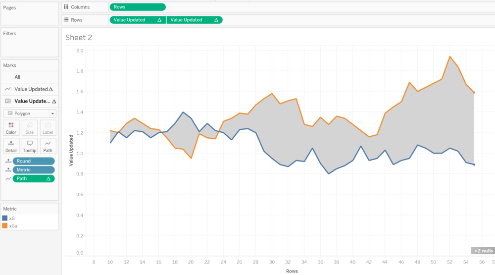
We can then place this field onto the Polygon field shelf and this creates the polygon bars which change colour depending on the difference between the round values.
The final view should look like this:
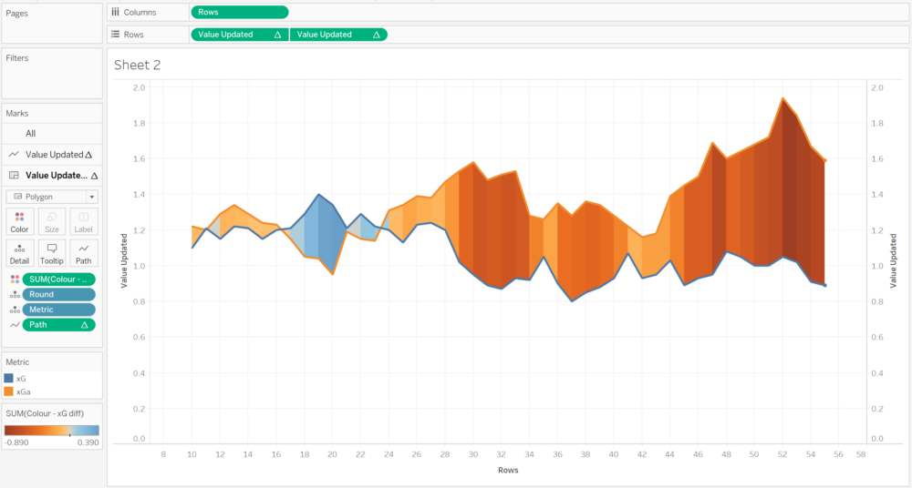
The darker the blue, the bigger the difference in favour of xG, and the darker the orange, the bigger the difference in favour of xGa.
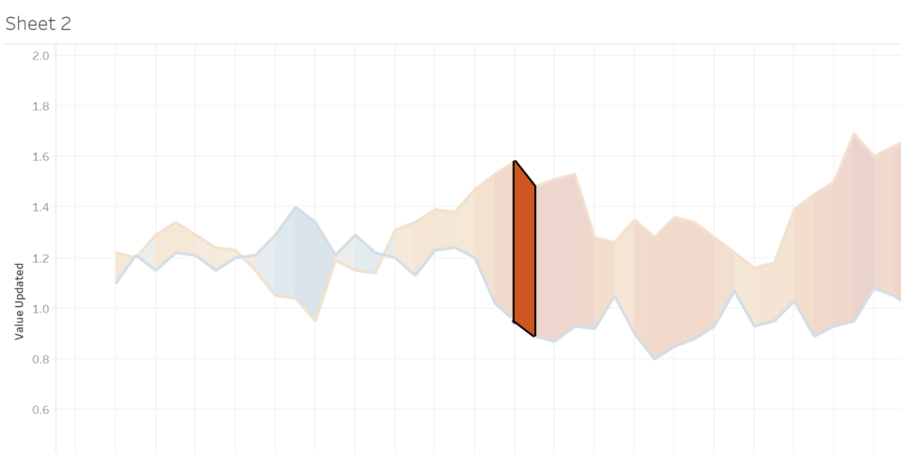
If I was to click on one of the bars, you can see how each one is an individual polygon and why we needed to make all of the changes with data structure and table calculations:
You can download the workbook from my Tableau Public here.
I took the methodology for this blog from the Tableau Public visualisation by Alexander Philipeit.
Another example visualisation can be found on my submission to #MakeoverMonday 2021 Week 1, where I have used this to see the difference in Bike usage between 2020 & 2019.
If you’re interested in learning more about Tableau then please get in touch via info@theinformationlab.co.uk and comment on this post if you have any questions!