

This is part 3, the final part, of my series on Table Calculations. If you haven't seen them I suggest you check out Part 1 and Part 2.In this part I want to return to the 'dynamic' small multiple / trellis chart I showed at the end of Part 1. Here it is again (or you can go a new window to see a larger version here):
This is based on a chart Marc Rueter showed in his talk (below) but I recreated it in my own way, so there's a few special differences (I hesitate to call them enhancements, judge for yourself). There's a lot going on here so I want to break it down and help make it accessible to newer users.1. Creating Dynamic Charts / DimensionsCreating Dynamic Charts - i.e. ones with a dimension / measure that is chosen by the user at run time - is one of the key aspects of this chart. It's simple once you know how - there's a great knowledge base article on doing this here.In my case I have created a parameter called Dimension
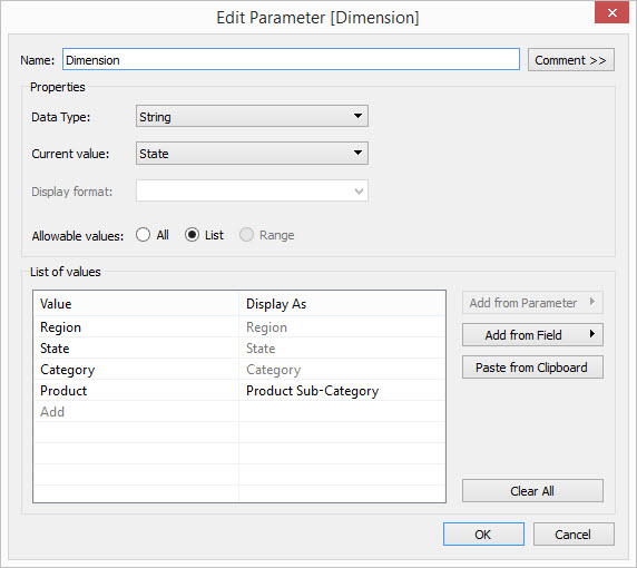 and an associated Calculated Field called [Dynamic Dimension]:
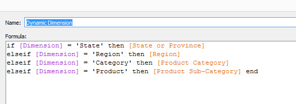 This calculation is just showing the associated dimension when needed.2. Splitting the Dimension over Different AxisOnce I'd built my chart I needed to create a way of determining where in my trellis each item was going to sit, to do this I needed to (a) find out the total number of dimension members there were and (b) find out the order of those dimensions so i could allocate them across the trellis. Hopefully if you've been playing attention to the previous posts then you'll recognise that the two calculations I need are SIZE() for (a) and INDEX() for (b).So now I need to calculate which row / column I want my dimension to fall in, if I have [m] members then I want them to be distributed across √ ( [m] ) rows and columns roughly. Here's the two calculations I chose.First the X axis, which determines the column:
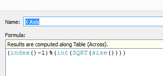 If you haven't come across the % sign then it is a modulus operator. Modulus is an operation that gives the remainder following division, i.e. 8 modulus 6 = 2 because 8/ 6 = 1 remainder 2. Another example, 15 modulus 7 = 1.So here we are calculating the INDEX() - 1, this gives us a zero-based position of our dimensions, then we take modulus with respect the square-root of the number of dimensions.So let's imagine we have 15 members, then our the square-root of 15 (to the nearest integer is 3) so:Item 1: (1-1) modulus 3 = 0Item 2: (2-1) modulus 3 = 1Item 3: (3-1) modulus 3 = 2Item 4: (4-1) modulus 3 = 0Item 5: (5-1) modulus 3 = 1Item 6: (6-1) modulus 3 = 2Item 7: (7-1) modulus 3 = 3Item 8: (8-1) modulus 3 = 0etcThis splits the columns up as we need to.next the rows, the Y Axis:
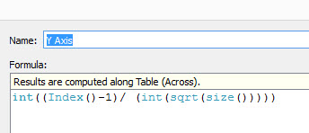 This is aAgain with our example:Item 1: int( (2-1) /3 ) = 0Item 2: int( (2-1) /3 )= int(1 / 3)= 0Item 3: int( (3-1) /3 )= int(2 / 3)= 0Item 4: int( (4-1) /3 )= int(3 / 3)= 1Item 5: int( (5-1) /3 )= int(4/ 3)= 1Item 6: int( (6-1) /3 )= int(5 / 3)= 1Item 7: int( (7-1) /3 )= int(6 / 3)= 2Item 8: int( (8-1) /3 )= int(7 / 3)= 2etcItem 15:int( (15-1)/3)= int(14/3)=4So note that we'll have 5 rows and 3 columns. This is slightly different to Marc's example (and a latter example by Dan Montgomery) where the columns and rows were more evenly distributed. For me this gives the line chart more room to 'breathe' but with the effect it squashes the y axis of the line chart, so there are trade-offs.3. Compute Using ProblemsI initially had problems when dropping on the X and Y Axis 'splitter' dimensions I had just built, the Compute Using I'd expect to work (Compute Using [Order Date]) just wasn't working. This led to some investigation, it led me to understanding a whole lot more about Table Calculations and it led to the previous two posts in this series - what a spin off from just this one visualisation! [Incidentally this is why I love blogging - it makes me understand what I'm writing].What was the problem? Well the [Order Date] variable consists of a different number of dates for each dimension member, i.e. some States didn't sell on a given date. This throws off the INDEX() calculation and affects the whole calculation of the X and Y splitters. How do you get round it? We explored it in detail in Part 2 of this series, but the 'At the level of' will ensure we get a kind of crosstab effect among the dimensions and those missing values will be populated for all dimension members.
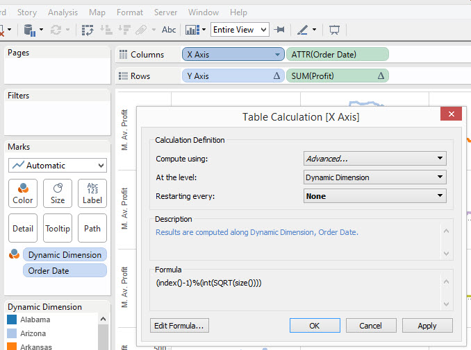 If you play around with this example and try to build it yourself, and I heartily recommend you do, you will also note the difference between using a discrete and a continuous variable in the table calculation. I need to do more experimentation here but it seems the Continuous variable doesn't let itself be 'padded' in the same way as the discrete version, so calculating using the Discrete version and using an ATTR on the continuous was a nice way to work around this - thanks to lots of older Tableau forum posts from Joe Mako for helping me figure out that one.At this stage we're done, and we can hide the headers for [X Axis] and [Y Axis]
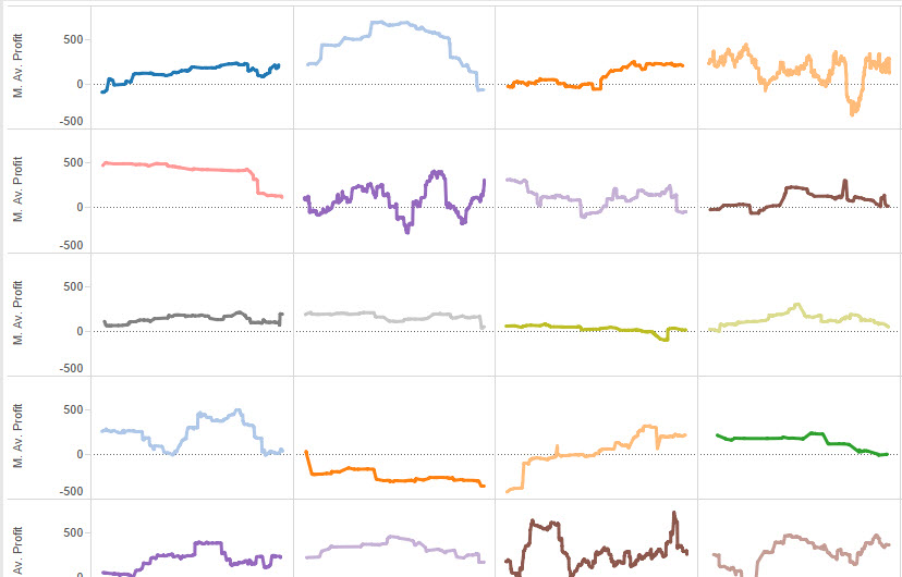 4. Adding a (optional) Title to each small multipleNow we have our Viz working we need to add a title, and boy this isn't as easy as I thought it might be. If we just add a label mark on [Dynamic Deminsion] Tableau will label the ends of the chart, but we want a nicer version in the middle of the chart don't we.Here's where I used a neat trick I've used many times before. A dummy variable called [One]:
 Not too complicated huh? I intend to do an entire blog post on the power of this calculated field but for now we just add it to the Viz as a new Row Dimension and we get this - the flat lines are the result of our new dimension.
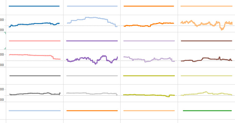 So now you're wondering where I'm going with this?Well I turned down the transparency to hide the line and added a new calculation:
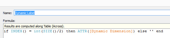 This calculates the point half way along each [Order Date] (by taking the number of [Dates], but wait...
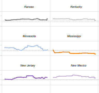 Hmm, not satisfactory. That INDEX() value sometimes occurs at different points making the titles wonky across the Viz - we need some uber calculation if we want to improve it. There are many solutions, here's mine (you'll need to click for a larger version)
![]() Not for the faint hearted! but it calculated the exact middle of each viz find the difference between the start and end dates, then finds the value that is closest to the date halfway between the two.That's it, a final touch if you wanted is to make the [One] variable dual axis to reduce the space taken by the header, as I have done on this second version.
Not for the faint hearted! but it calculated the exact middle of each viz find the difference between the start and end dates, then finds the value that is closest to the date halfway between the two.That's it, a final touch if you wanted is to make the [One] variable dual axis to reduce the space taken by the header, as I have done on this second version.