9 March 2018

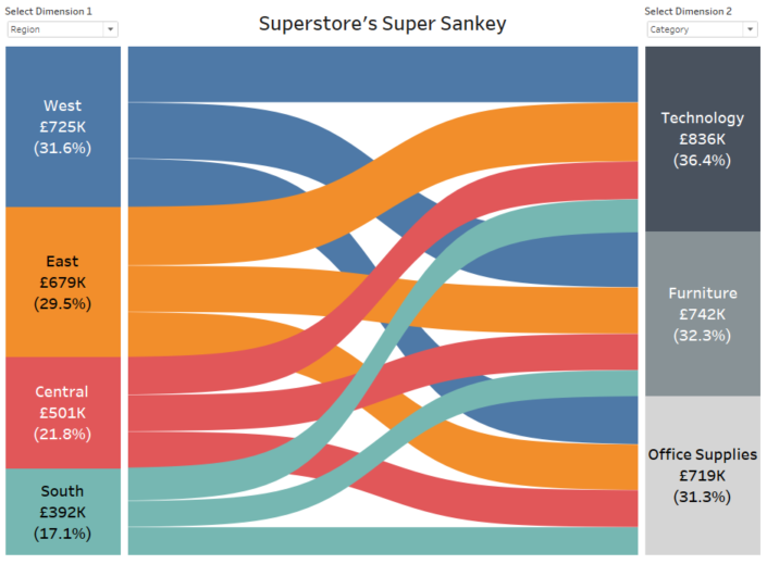
First of all I want to say this post is hugely indebted to Olivier Catherin and his post four years ago on building Sankeys in Tableau and Jeff Schaffer whose work Olivier built off and countless others I probably don't even realise.This post sets out how to build a Sankey Diagram without any data prep before Tableau. The viz below is built off the vanilla Superstore data packaged with Tableau, but I must warn you there's a labyrinth of table calculations to get to this point.[iframe src='https://public.tableau.com/views/SuperstoresSuperSankey/Dashboard1?:embed=y&:display_count=yes&:showVizHome=no&:tabs=no' width='650px' height='650px' scrolling='no']There are 20 calculations to get through to get to this stage so what makes it worth it? All previous solutions I've seen for building Sankeys have needed to multiply the size of the data by at least a factor of two beforehand. Some data sets are so large that we don't want to do that and sometimes we come across data sources such as published data sources on Tableau Server where we're not the owners and this isn't an option. So if we can work off the vanilla data set it'd be worth the effort.So without further ado let's get going.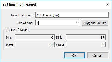
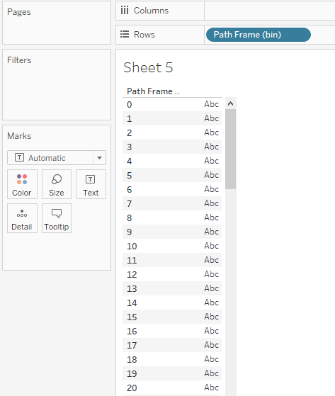
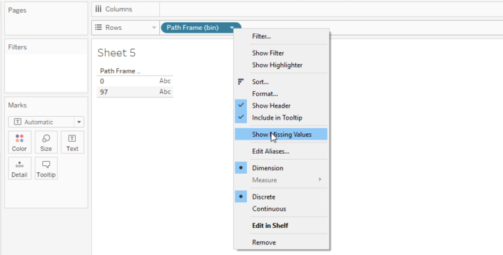 This should give you something like below. This is the step that enables our data densification within Tableau.
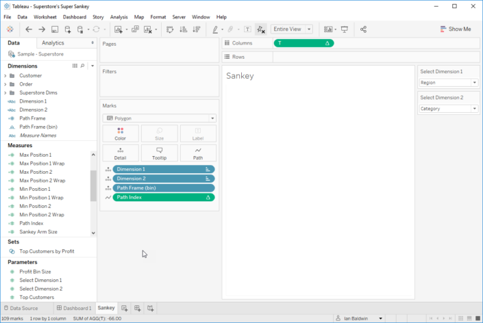
 Then move Path Frame (bin) to detail and add Dimension 1 and Dimension 2 to detail too. Next, put [T] on Columns and calculate it along Path Frame (bin). Finally change mark type to Polygon, and add [Path Index] to path and calculate it along Path Frame (bin). This should leave you with something like this:
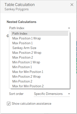 Below I've shown the settings for each of the 12 nested calculations to make this work. If it doesn't look right at the end, make sure that not only the correct fields are ticked in each box but that they're ordered correctly as well.
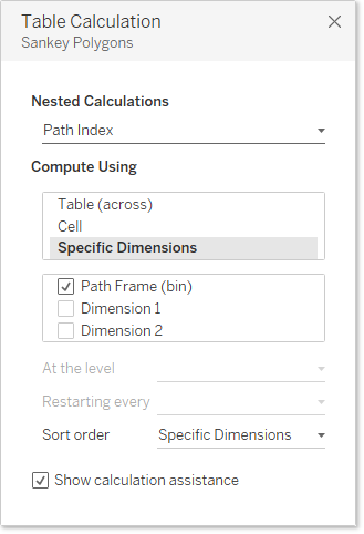

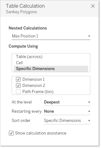
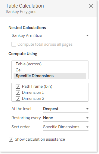
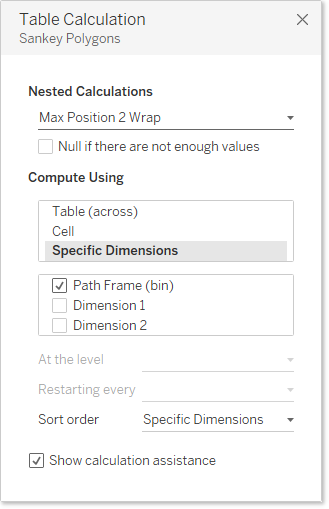
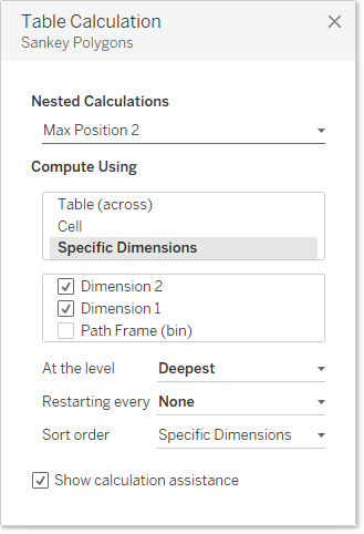

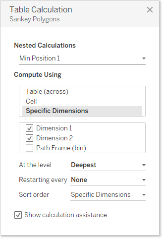
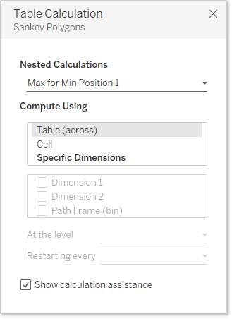


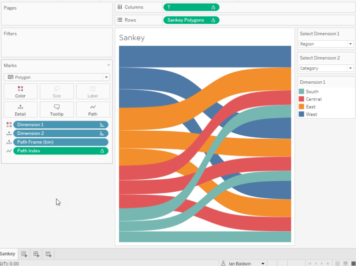
 Now hopefully you have something that looks like this! (If not go back and check each table calculation step carefully)
 I hope you've made it to the end and have been able to replicate this Sankey. Thanks for reading :)
Step 1: Dimension and measure parameterisation
Set up 3 calculations, 2 for your dimensions and 1 for your measure. It's useful down the line to reference these in case you want to change which dimensions you want in the view part way through building and you can edit the calcs rather than fiddling with 'replace references'. In my example I used these calculations where [Select Dimension 1] and [Select Dimension 2] are parameters I made to fit the case statement:Dimension 1
CASE [Select Dimension 1]WHEN 1 THEN [Region]WHEN 2 THEN [Category]WHEN 3 THEN [Sub-Category]WHEN 4 THEN [Segment]WHEN 5 THEN [Ship Mode]ENDDimension 2
CASE [Select Dimension 1]WHEN 1 THEN [Region]WHEN 2 THEN [Category]WHEN 3 THEN [Sub-Category]WHEN 4 THEN [Segment]WHEN 5 THEN [Ship Mode]ENDChosen Measure
[Sales]Step 2: Create a frame for data densification
Comparing our measure to the fixed min of the measure we can ensure two data points to hang our data densification from.Path Frame
IF [Chosen Measure] = {FIXED : MIN([Chosen Measure])} THEN 0 ELSE 97 ENDPath Frame (bin)
For this create bins of size 1 from Path Frame
Step 3: Index
Path Index
Index()This is computed along Path Frame (bin) and allows us to do calculations across the Path Frame range.Step 4: Sigmoid set up
First we have a variable, T, and then the sigmoid curve is calculated using it.T
IF [Path Index] < 50THEN (([Path Index]-1)%49)/4-6ELSE 12 - (([Path Index]-1)%49)/4-6ENDSigmoid
1/(1+EXP(1)^-[T])Step 5: Sankey arm sizing
This gives us the size of each Sankey arm as a percentage of the full data set.Sankey Arm Size
SUM([Chosen Measure])/TOTAL(SUM([Chosen Measure]))Step 6: Top line calculations
This method requires separate lines for the top and bottoms of each Sankey arm and throughout these calculations 'Position 1' will refer to Dimension 1 on the left hand side and 'Position 2' to Dimension 2 on the right. Here are the calculations for the tops:Max Position 1
RUNNING_SUM([Sankey Arm Size])Max Position 1 Wrap
WINDOW_SUM([Max Position 1])Max Position 2
RUNNING_SUM([Sankey Arm Size])Max Position 2 Wrap
WINDOW_SUM([Max Position 2])Step 7: Bottom line calculations
These calculations help generate the bottom lines:Max for Min Position 1
RUNNING_SUM([Sankey Arm Size])Min Position 1
RUNNING_SUM([Max for Min Position 1])-[Sankey Arm Size]Min Position 1 Wrap
WINDOW_SUM([Min Position 1])Max for Min Position 2
RUNNING_SUM([Sankey Arm Size])Min Position 2
RUNNING_SUM([Max for Min Position 2])-[Sankey Arm Size]Min Position 2 Wrap
WINDOW_SUM([Min Position 2])Step 8: Sankey polygon calculation
This calculation brings together all of the above once set up correctly. The table calculation set up itself will come in later steps.Sankey Polygons
IF [Path Index] > 49THEN [Max Position 1 Wrap]+([Max Position 2 Wrap]-[Max Position 1 Wrap])*[Sigmoid]ELSE [Min Position 1 Wrap]+([Min Position 2 Wrap]-[Min Position 1 Wrap])*[Sigmoid]ENDStep 9: Prepare the sheet
Put Path Frame (bin) onto Rows, then right click it and select 'show missing values' as below This should give you something like below. This is the step that enables our data densification within Tableau.
 Then move Path Frame (bin) to detail and add Dimension 1 and Dimension 2 to detail too. Next, put [T] on Columns and calculate it along Path Frame (bin). Finally change mark type to Polygon, and add [Path Index] to path and calculate it along Path Frame (bin). This should leave you with something like this:
Step 10: Add Sankey polygons
Add [Sankey Polygons] to Rows. This is going to look a bit messy until it is calculated correctly across all nested calculations.This first image shows all of the nested calculations involved and we need to go through each one setting them up correctly. Below I've shown the settings for each of the 12 nested calculations to make this work. If it doesn't look right at the end, make sure that not only the correct fields are ticked in each box but that they're ordered correctly as well.


 Now hopefully you have something that looks like this! (If not go back and check each table calculation step carefully)
Step 11: Dashboarding
Now we're ready to put this onto a dashboard with stacked bars either side for dimensions 1 and 2 to complete our Sankey.This graph is filterable if you want it to be, just make sure they are on context so that they happen before the Fixed LOD calculation in Tableau's order of operations, otherwise the filters might knock out the Path Frame calculation that all of this hinges upon. I hope you've made it to the end and have been able to replicate this Sankey. Thanks for reading :)