20 July 2015
In the first blog in this series (Joining Excel Worksheets) I touched upon the required structure of a CSV or Excel file to be able to maximize the potential of the data, to analyse the data at its most granular level and for us to visualize our data using Tableau (more information on this here).So what if our data isn’t in the required format, what if we have workbooks upon workbooks that contain cross-tabs?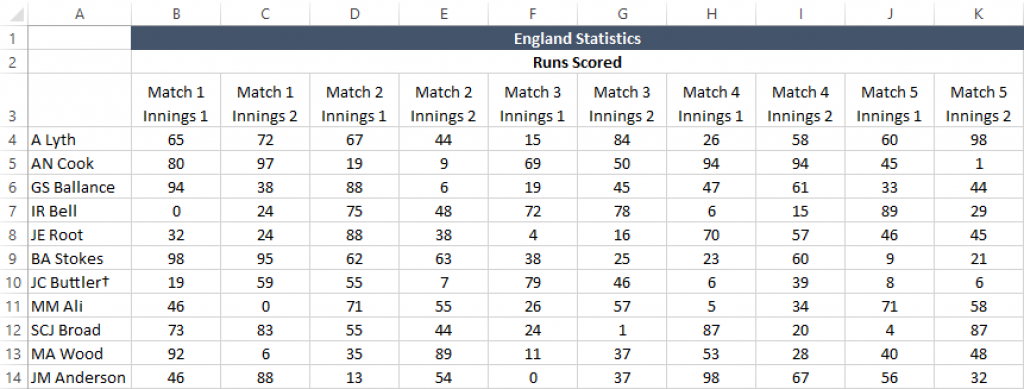
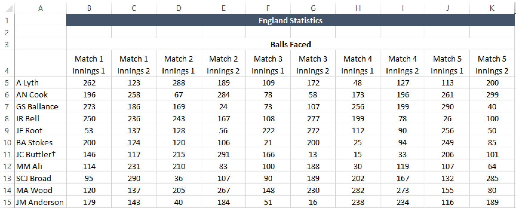
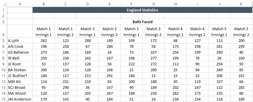 The first thing to note is that each worksheet contains a cross-tab (table of data) along with header rows and a title within the worksheet. The second factor to note is that the “Balls Faced” worksheet also has an additional blank row in row 2.This formatting and the minor differences between workbooks (ie. additional blank row) is a common feature of many Excel workbooks that exist in sports clubs, usually due to different people editing them or even just a lack of understanding and appreciation towards the importance of a standardized format.Now let’s start the process of turning these two separate cross-tabs in to one single comprehensive database (note: you could do this with as many different cross-tabs as you desire) .
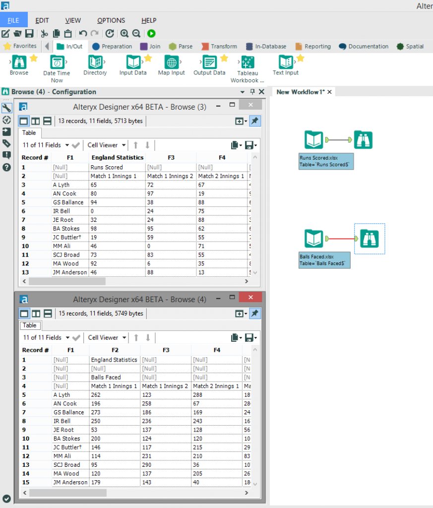 First we use two “Input Data” tools and connect to the “Runs Scored” and “Balls Faced” worksheets.I have added a “Browse” tool after each input, this enables you to preview the data coming through the workflow. You can see in the above example that, due to the different structure of each Excel worksheet, the “Browse” tool shows two slightly differently structured outputs.Also note that the first row of data from the excel workbooks has been identified as a header in the “Runs Scored” worksheet but as the first row of data in the “Balls Faced” worksheet.Next we need to remove the unwanted rows at the top of our cross-tab - for this we can use the “Sample” tool. Connect your “Input Data” tools to the respective “Sample” tools and select “Skip 1st N Records” in the configuration. On the “Runs Scored” data we need to set N=1 and on the “Balls Faced” data we need to set N=3 to account for the additional blank row and the fact that no header row was identified when connecting to that data.
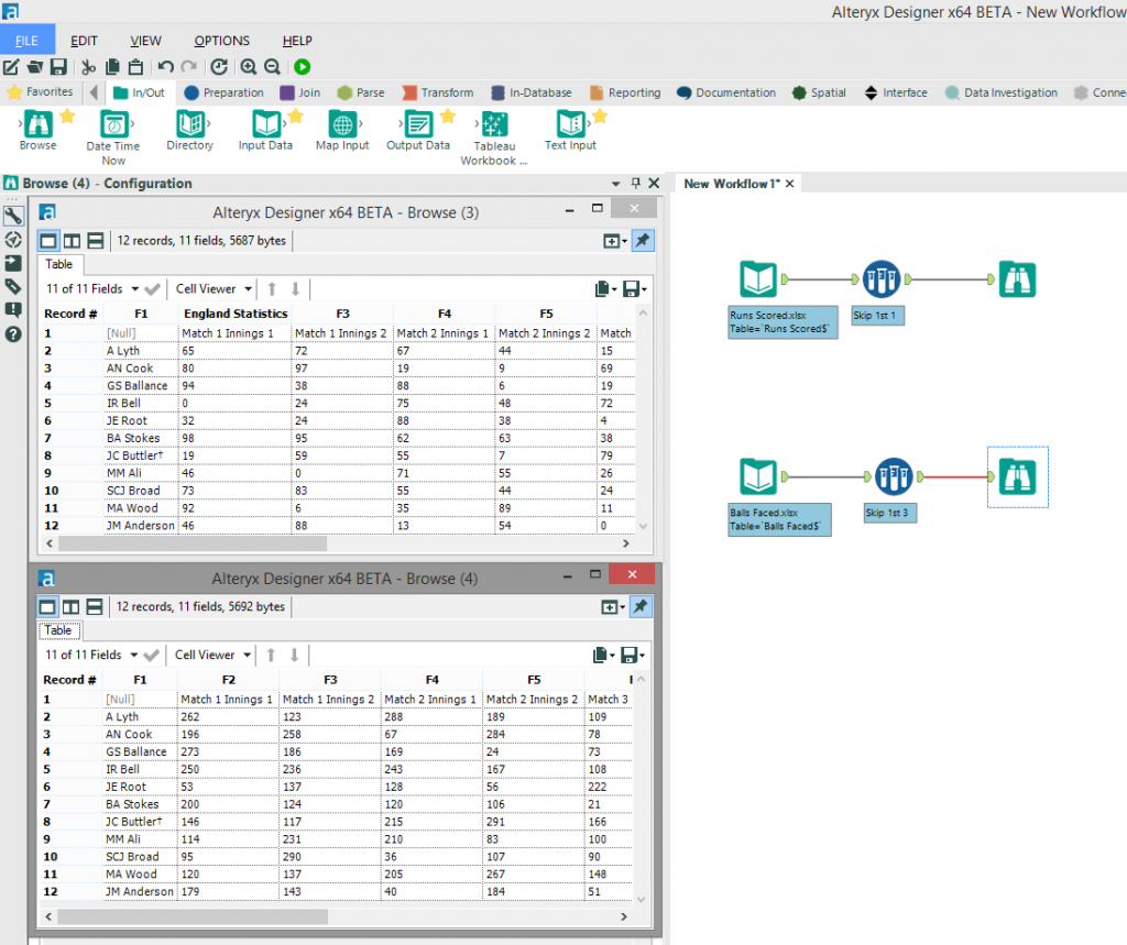 You will see in the browse windows (screenshot above) that we have now removed the unwanted rows but are left we the header rows as the first row of data. This is where we introduce our next tool to the workflow, the “Dynamic Rename” tool.Using the “Dynamic Rename” tool we are able to quickly rename any or all of the fields within the input stream using a variety of methods. In this instance we are going to choose the “Take Field Names from First Row of Data” mode from the drop-down selection in the configuration window. This will rename the fields with the data from the first row (as can be seen in the browse windows below).
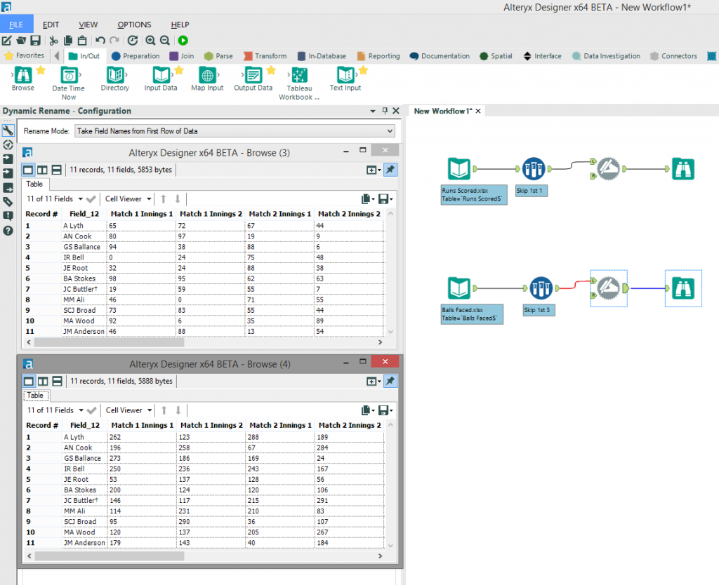 We can then use the “Select” tool to rename the field “Field_12” to “Player” to give it a clearer meaning.
 The next step is to turn each of our cross-tabs into the row-by-row structure we initially wanted. Using the “Transpose” tool we can reshape the data and pivot the cross-tab. Our key field in this instance is the “Player” with all of the matches/innings being the data fields.
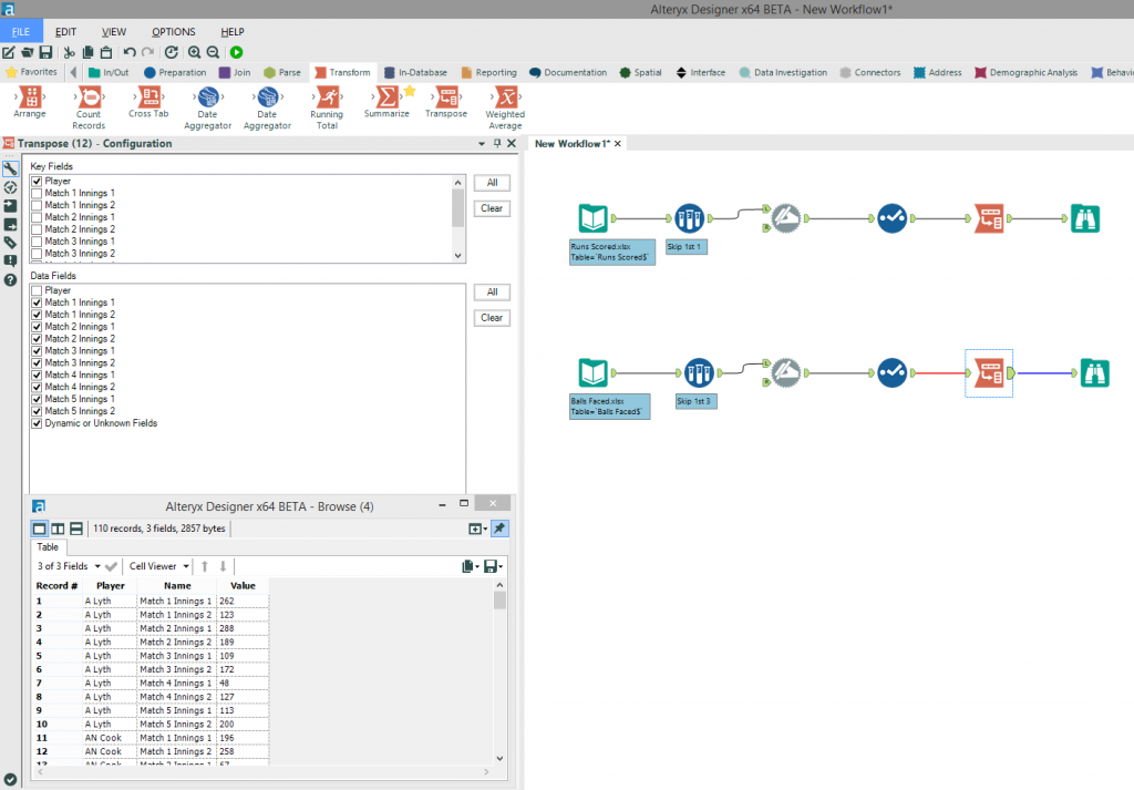 So now we have our two original cross-tabs in the structure we want, all we need to do now is join the two data streams to provide us with the comprehensive database we require. To do this we will use the “Join” tool. This enables us to join two data streams together on specified fields, which in this case is “Player” and “Name” (which is the match/innings name). I will also take this opportunity to use the rename and type options in the “Join” tool’s configuration to change the Runs Scored and Balls Faced fields to the correct name and to be integers.
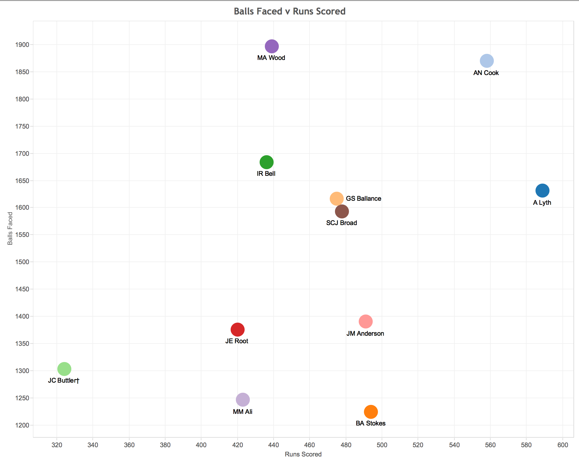
 All we need to do then is to export our data to the required file (in this case a .tde) and there we have it. In one short workflow we have taken two related cross-tabs from two separate Excel workbooks with slightly different structures and combined them in to one database that will enable us to gain a deeper understanding of our metrics and their relationship with each other.
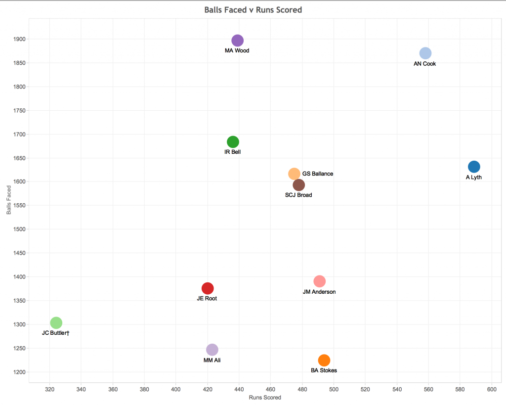
When cross-tab meets Alteryx
Reshaping our Excel data is a breeze when using Alteryx, no opening of multiple workbooks, no vlookups and no copy and pasting, just a few drag-and-drop tools between you and your insights.In the below example we have two excel workbooks with (made-up) cricket data; one worksheet that contains runs scored and one worksheet that contains balls faced.
 The first thing to note is that each worksheet contains a cross-tab (table of data) along with header rows and a title within the worksheet. The second factor to note is that the “Balls Faced” worksheet also has an additional blank row in row 2.This formatting and the minor differences between workbooks (ie. additional blank row) is a common feature of many Excel workbooks that exist in sports clubs, usually due to different people editing them or even just a lack of understanding and appreciation towards the importance of a standardized format.Now let’s start the process of turning these two separate cross-tabs in to one single comprehensive database (note: you could do this with as many different cross-tabs as you desire) .
 First we use two “Input Data” tools and connect to the “Runs Scored” and “Balls Faced” worksheets.I have added a “Browse” tool after each input, this enables you to preview the data coming through the workflow. You can see in the above example that, due to the different structure of each Excel worksheet, the “Browse” tool shows two slightly differently structured outputs.Also note that the first row of data from the excel workbooks has been identified as a header in the “Runs Scored” worksheet but as the first row of data in the “Balls Faced” worksheet.Next we need to remove the unwanted rows at the top of our cross-tab - for this we can use the “Sample” tool. Connect your “Input Data” tools to the respective “Sample” tools and select “Skip 1st N Records” in the configuration. On the “Runs Scored” data we need to set N=1 and on the “Balls Faced” data we need to set N=3 to account for the additional blank row and the fact that no header row was identified when connecting to that data.You will see in the browse windows (screenshot above) that we have now removed the unwanted rows but are left we the header rows as the first row of data. This is where we introduce our next tool to the workflow, the “Dynamic Rename” tool.Using the “Dynamic Rename” tool we are able to quickly rename any or all of the fields within the input stream using a variety of methods. In this instance we are going to choose the “Take Field Names from First Row of Data” mode from the drop-down selection in the configuration window. This will rename the fields with the data from the first row (as can be seen in the browse windows below).
 We can then use the “Select” tool to rename the field “Field_12” to “Player” to give it a clearer meaning.
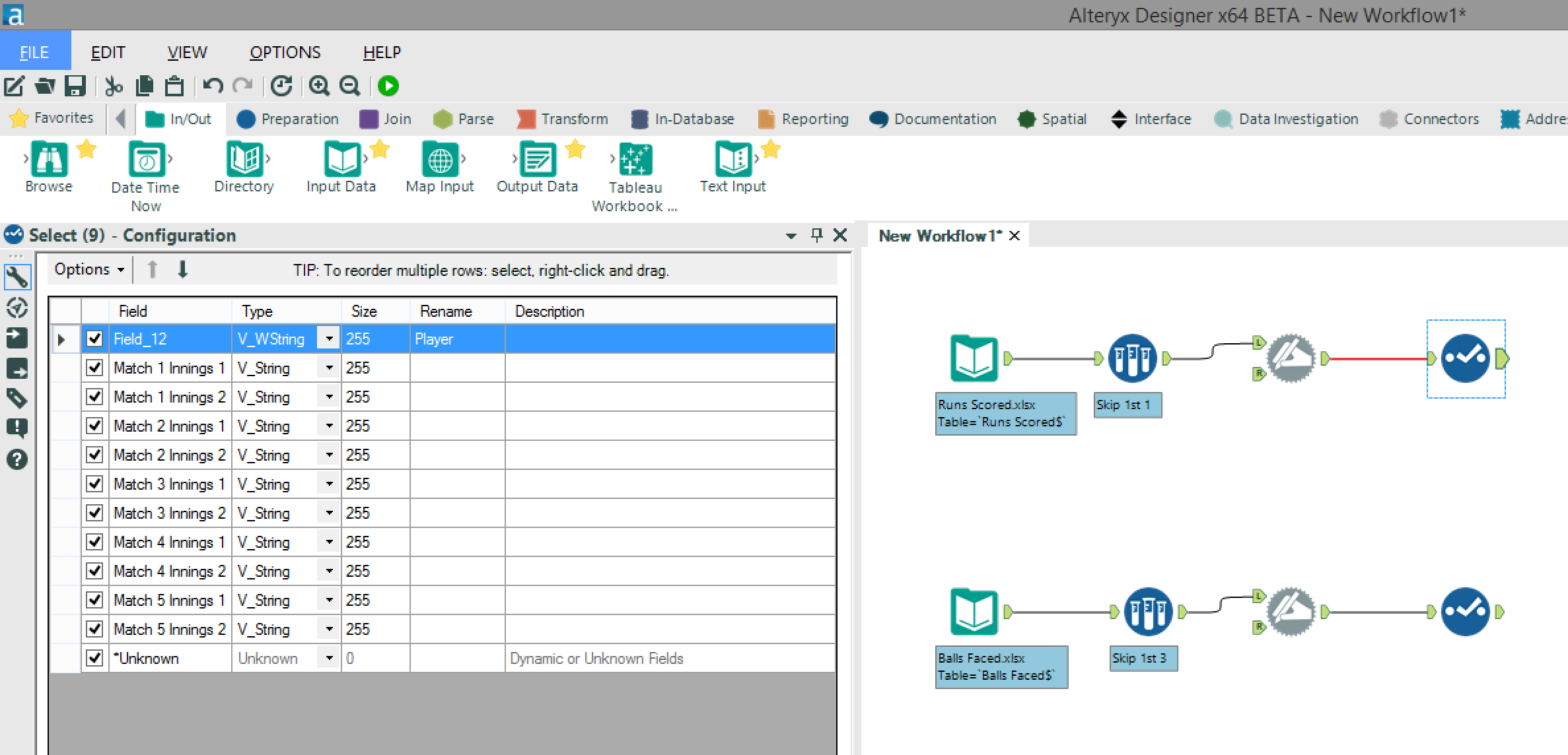 The next step is to turn each of our cross-tabs into the row-by-row structure we initially wanted. Using the “Transpose” tool we can reshape the data and pivot the cross-tab. Our key field in this instance is the “Player” with all of the matches/innings being the data fields.
 So now we have our two original cross-tabs in the structure we want, all we need to do now is join the two data streams to provide us with the comprehensive database we require. To do this we will use the “Join” tool. This enables us to join two data streams together on specified fields, which in this case is “Player” and “Name” (which is the match/innings name). I will also take this opportunity to use the rename and type options in the “Join” tool’s configuration to change the Runs Scored and Balls Faced fields to the correct name and to be integers.
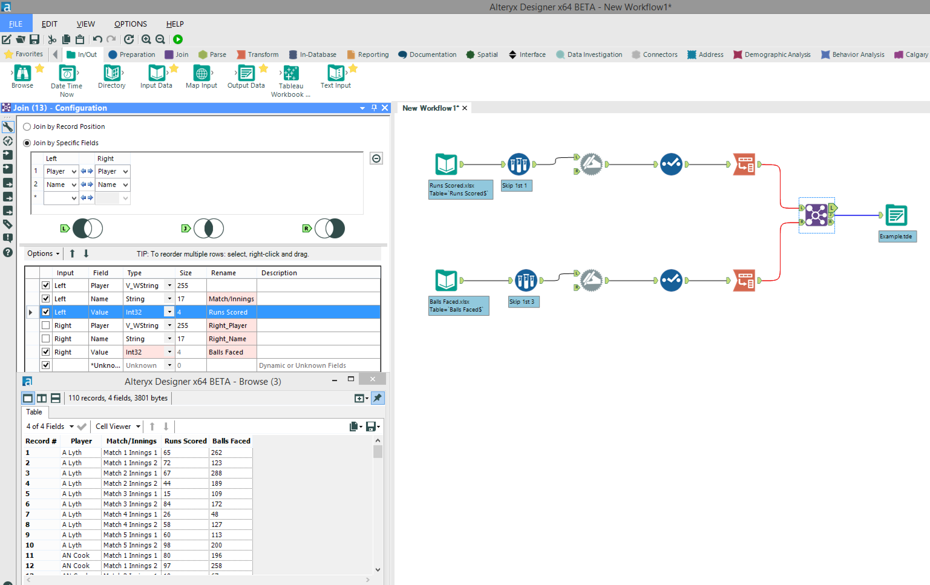 All we need to do then is to export our data to the required file (in this case a .tde) and there we have it. In one short workflow we have taken two related cross-tabs from two separate Excel workbooks with slightly different structures and combined them in to one database that will enable us to gain a deeper understanding of our metrics and their relationship with each other.